
How to create a range of numbers in Excel – 3 easy ways


Table of Contents
If you’re wondering how to create a range of numbers in Excel, we’ve got you covered right here with a few methods you can use.
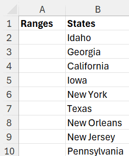
Here’s the example we’re using for this guide. A list of states in a table.
Prime Day is finally here! Find all the biggest tech and PC deals below.
- Sapphire 11348-03-20G Pulse AMD Radeon™ RX 9070 XT Was $779 Now $739
- AMD Ryzen 7 7800X3D 8-Core, 16-Thread Desktop Processor Was $449 Now $341
- ASUS RTX™ 5060 OC Edition Graphics Card Was $379 Now $339
- LG 77-Inch Class OLED evo AI 4K C5 Series Smart TV Was $3,696 Now $2,796
- Intel® Core™ i7-14700K New Gaming Desktop Was $320.99 Now $274
- Lexar 2TB NM1090 w/HeatSink SSD PCIe Gen5x4 NVMe M.2 Was $281.97 Now $214.98
- Apple Watch Series 10 GPS + Cellular 42mm case Smartwatch Was $499.99 Now $379.99
- ASUS ROG Strix G16 (2025) 16" FHD, RTX 5060 gaming laptop Was $1,499.99 Now $1,274.99
- Apple iPad mini (A17 Pro): Apple Intelligence Was $499.99 Now $379.99
*Prices and savings subject to change. Click through to get the current prices.
As you can see, the States are in Column B and space for a list of different Ranges in Column A. For this example, let's say we want to quickly create a range of numbers for the list of States.
Method 1 – Using the FILL function
In this method, we will use the FILL function to create a range of sequential numbers in Excel.
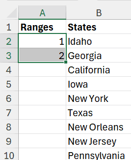
- Enter the first 2 numbers in the sequence in the first 2 rows as shown below. For this example, we will place the numbers 1 in cell A2 and 2 in cell A3.
- Next, we will place the cursor over cells A2 and A3 as shown below.
- Next, we will hover over the edge of the green box until a plus sign appears on the right, bottom corner as shown below.
- Then we will double-click the plus sign to create a sequential range of numbers as shown in the video below.
Method 1 applies to any sequence of numbers you prefer, for example, if you prefer to have the sequence multiplied by six each time, simply start with two numbers in a six-digit interval as shown in the video below.
Method 2 – Using the RANDBETWEEN function.
In this method, we will use the RANDBETWEEN function to create a random range of numbers in Excel.
Steps:
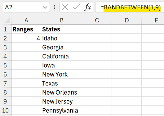
- Select the cell you want the first number to appear. For this example, the cell will be A2.
- Enter the function = RANDBETWEEN then select the lowest and highest number in the count of the States list in Column B, which will be the numbers 1 and 9. Add numbers 1 and 9 in parenthesis to the RANDBETWEEN function as shown below.
- Then we will double-click on the plus sign to create a random range of numbers as shown in the video below.
Method 3 – Using the SERIES function.
In this method, we will use the SERIES function to create a specified sequence of numbers in Excel.
Steps:
- Select the cell you want the first number to appear. For this example, the cell will be A2.
- Enter the number you want to start the sequence with. For this example, the number will be 1.
- From the Home tab, select the SERIES function from the Home tab's Editing section.
- Ensure both Column and Linear are selected.
- Then select the number sequence of your choice. For this example, the sequence should increase by 3 until the number reaches 25. Therefore, 3 should be entered in the step value box and 25 should be entered in the stop value box and select OK as shown below.
- To review the steps for Method 3 again please watch the video below.
Conclusion
So there you have it, three different methods to create ranges of numbers in Excel. For more tips, tricks, and guides to everything Excel, be sure to check back in with us soon.
About the Author