How to ignore all errors in Excel – 5 easy methods

If you want to learn how to ignore all errors in Excel, then we have a handful of methods for you.

While working in Excel, you are bound to encounter various issues and errors. If you’re entering the wrong formula, the error can be indicated by a #VALUE! or a #NAME! message. On the other hand, if Excel finds some discrepancy in the formula, the error will be indicated by a little green triangle in the upper-left corner of a cell.

While automated error identification can help you in your Excel tasks, at times, the error marks can become very annoying. In this guide, you will learn how to ignore errors in Excel through a sample dataset. 

How you can ignore errors in Excel

Scenario on hand: We have a product dataset in Excel.  

What we want to accomplish: Explore how to ignore formula and green triangle errors in Excel using the following ways:

1. Ignore the error with the shortcut menu
2. Ignore the error in a range
3. Turn off error-checking options
4. Set error-checking rules
5. Use the IFERROR function

Ignore the error with the shortcut menu

Ignoring errors in specific cells is easy. All you have to do is select the cell and open up a shortcut menu to select the “Ignore error” option. 

To explain this better, let’s get on with the demonstration. 

Step 1: Select the cell with the error

We have an Excel dataset with product names, prices, and tax calculations. 

Note that there are green triangles in all the cells where we calculated the tax on the product price in column F. 

Since the formula is correct, Excel has calculated the tax on each product price. However, since the tax percentage was taken from a cell outside of the table, Excel has detected it as a possible error. 

The first step is to select a cell in the column where Excel has marked a green triangle. 

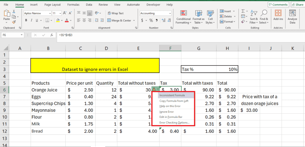
Upon selecting the column, we get an icon – a triangle marked with an exclamation mark:

Step 2: Open the shortcut menu

To see more details on the error or ignore the error, click the triangle icon. Here’s what you will get:

The first option on the list tells you the error type. Here, the error is an “Inconsistent formula.”

To ignore the error, select Ignore Error from the menu. 

After you ignore the error, Excel will remove the green triangle from the top left corner of the cell:

Sometimes, you may have to ignore errors in specific cells. To do this, you can simply drag the selected cells with a green triangle. Click the Trace Error option and choose Ignore Error from the shortcut menu.

This option lets you ignore errors located in the certain cells you have selected. You will not see the green triangle once you have selected ignore the error.

Ignore the error in a range

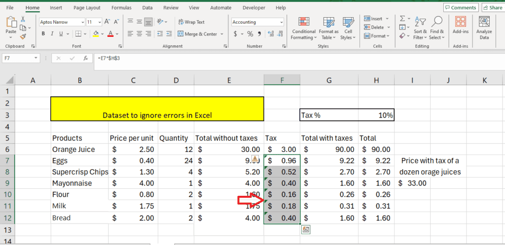
To ignore the error through the shortcut menu in a range, instead of selecting every cell individually, simply select the entire range and click on the Error triangle icon to ignore the error in every cell of the range:

Step 1: Select the range

The first step is selecting the range with the error marks.

Step 2: Ignore error

Click the triangle error icon to open the shortcut menu and select Ignore error.

Excel will now remove all error marks from the range. 

Turn off error-checking options

The error-checking option is helpful for people handling a lot of data in Excel. However, if you wish, you can turn off error-checking in Excel from the settings. Here are the steps to follow for this method to ignore errors in Excel:

Step 1: Go to options

Click the File tab from the top ribbon. Here, click More…> Options.

Step 2: Disable error-checking

Upon clicking Options, a window will open. 

In the window, select Formulas and disable error checking by unchecking the option Enable background error checking.

You have now disabled background error-checking in Excel, and it will not mark any cells with the green triangle till you enable this option again. 

Select error-checking rules

Error-checking on Excel might save you from a lot of human errors. However, some error rules on Excel mark even those cells with no apparent errors. In this case, it is best not to turn off error-checking completely but to modify the error-changing rules. Here’s how you do it:

Step 1: Go to Options

Click the File tab from the top ribbon. Here, click More…> Options.

Step 2: Disable selected error rules

From the menu that pops up, disable the error rules that you don’t feel are relevant to you:

Use the IFERROR function

Many times, inputting the wrong formula might also get you error messages like these:

1. #VALUE!
2. #NAME!
3. #REF!
4. #DIV/O!
5. #N/A!
6. #NULL!

While every error type refers to a different kind of error, to avoid displaying an error, you can use the IFERROR function by following these steps:

Step 1: Enter a formula

The first step is entering the formula.

Because the number is divided by zero, we get a #DIV/O! error in the cell:

Step 2: Add IFERROR to the formula

The second step is to add IFERROR to the formula. 

Here’s the formula we had originally:

=I9/I10

We added IFERROR to this formula like this:

=IFERROR (I9/I10, “Error here”)

Here’s the syntax for the IFERROR formula:

=IFERROR (<Original formula>, “<Value if error>”)

Here’s what we get by adding IFERROR to the original formula in our scenario:

How to ignore selected errors in Excel?

You can choose to ignore selected errors in Excel by clicking the cell with the green triangle marked on the top left corner and selecting “Ignore Error” from the shortcut menu. Alternatively, you can modify the error-checking rules in Excel by going to File> More> Options > Formulas. 

How do you use the IFERROR function in Excel?

To use the IFERROR function in Excel, add IFERROR in front of the formula, enter the formula as the first entry in the formula bracket, and add the return value as the second entry in the formula bracket.

Wrapping up

There will be many times when you want Excel to ignore errors in your workbook. There are multiple ways to ignore the error. You can either ignore the error cell by cell, select a range, ignore the error from the shortcut menu, disable error checking completely, modify the error checking rules, and use the IFERROR function. 

We hope this article has helped you find the right way to resolve your error issue.

If you have any other cool tricks you use to ignore errors in Excel, share them with us in the comments below! We would love to feature your trick in our next article.