
How to use VLOOKUP to search text in Excel – 5 easy ways


Table of Contents
Want to know how to use VLOOKUP to search text in Excel? We’ve got you covered right here.
Let's say you have a product dataset with their codes, names, and categories. Now, you want to look up products using keywords. Manually looking through a huge dataset would take a lot of work. You could use the Ctrl+F function to search for text. But if you're doing this for a range of lookup keywords, using Ctrl+F is not the way to go.
Prime Day may have closed its doors, but that hasn't stopped great deals from landing on the web's biggest online retailer. Here are all the best last chance savings from this year's Prime event.
- Sapphire 11348-03-20G Pulse AMD Radeon™ RX 9070 XT Was $779 Now $719
- AMD Ryzen 7 7800X3D 8-Core, 16-Thread Desktop Processor Was $449 Now $341
- Skytech King 95 Gaming PC Desktop, Ryzen 7 9800X3D 4.7 GHz Was $2,899 Now $2,599
- LG 77-Inch Class OLED evo AI 4K C5 Series Smart TV Was $3,696 Now $2,996
- AOC Laptop Computer 16GB RAM 512GB SSD Was $360.99 Now $306.84
- Lexar 2TB NM1090 w/HeatSink SSD PCIe Gen5x4 NVMe M.2 Was $281.97 Now $214.98
- Apple Watch Series 10 GPS + Cellular 42mm case Smartwatch Was $499.99 Now $379.99
- AMD Ryzen 9 5950X 16-core, 32-thread unlocked desktop processor Was $3199.99 Now $279.99
- Garmin vívoactive 5, Health and Fitness GPS Smartwatch Was $299.99 Now $190
*Prices and savings subject to change. Click through to get the current prices.
VLOOKUP is a handy formula to use in Excel, as its functionalities allow you to detect text errors and even report parts of text. In this guide, we’ll walk you through how you can use this function to search text in Excel.
How you can use VLOOKUP to search text in Excel
Here’s the scenario – we have a sample product dataset with their code, name, and category.
Let's explore the following five ways to use VLOOKUP to search for text in a dataset in Excel.
- Searching for text using text via the VLOOKUP formula
- Finding text using cell address through the VLOOKUP formula
- Searching for the presence of text value among numbers using the VLOOKUP formula
- Using VLOOKUP to search for the corresponding text
- Using LEFT and RIGHT VLOOKUP functions to search for matching text
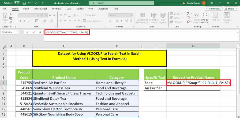
Method 1 – Searching for text using text via the VLOOKUP formula
We can use the VLOOKUP formula to search for specific text by entering the text in the formula. To proceed:
1. Choose a cell where you want the lookup output and then enter the following formula:
=VLOOKUP(“*{Text you want to search}*”, {Two column table range}, {1 or 2}, {FALSE})
=VLOOKUP(“*Soap*”, C7:D13, 1, FALSE)
Side-notes:
- Here, you need to enter the table range of two columns since the formula only works for a 2 column dataset.
- 1 or 2 is the column index number which contains the text you want to search for.
- False or True is for an exact match or an approximate match. We put FALSE in the formula since we want an exact match of the text we entered.
2. Hit Enter to see the results.
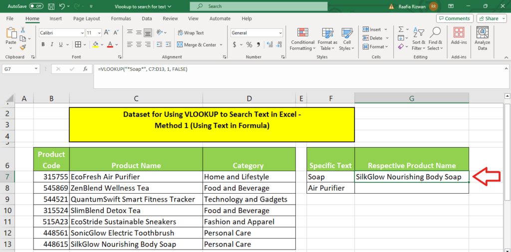
That was the easiest way to look for a specific text within a dataset using the VLOOKUP formula.
With this formula, you cannot use the Fill Handle drag tool to get results automatically in the remaining cells. For that, we use a formula with the cell address in place of the text.
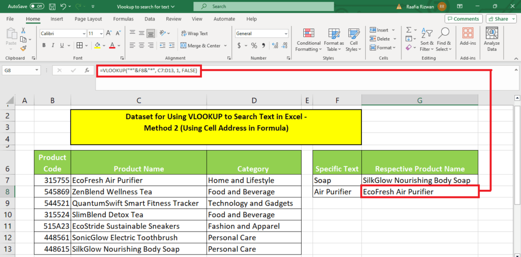
Method 2 – Finding text using cell address through the VLOOKUP formula
We can use the VLOOKUP formula to search for specific text by entering the cell address in the formula. To proceed:
1. Choose a cell where you want the lookup output and then enter the following formula:
=VLOOKUP(“*”&{Cell Address}&”*”, {Two column table range}, {1 or 2}, {FALSE})
=VLOOKUP(“*”&F8&”*”, C7:D13, 1, FALSE)
Method 3 – Searching for the presence of text value among numbers using the VLOOKUP formula
At times, due to errors, you might have a text value within numeric data. The VLOOKUP formula comes in handy to identify such issues.
1. Enter the following formula in any cell and press enter:
=VLOOKUP(“*”,{Lookup range},{1 or 2} ,{FALSE})
=VLOOKUP(“*”,B7:B13,1,FALSE)
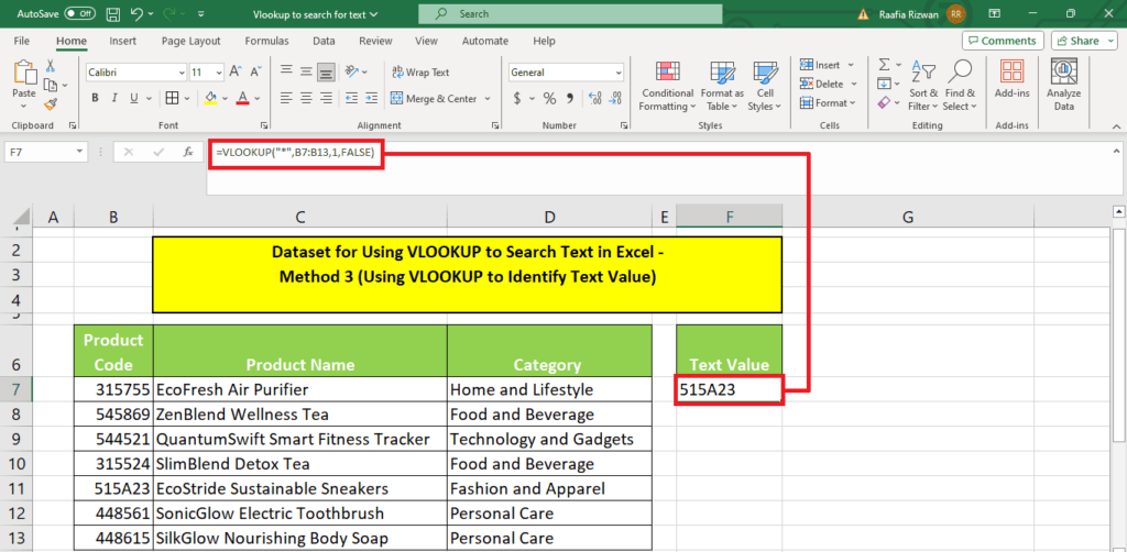
This formula helps us to identify the error in the product codes.
Method 4 – Using VLOOKUP to search for the corresponding text
This method uses the VLOOKUP formula to search for corresponding text in a dataset.
1. Type this formula in your output table:
=VLOOKUP({String or numeric lookup value}, {Dataset range with $ sign}, {Column index number}, {TRUE or FALSE})
=VLOOKUP(F7, $B$7:$D$13, 2, FALSE)
Next, press Enter.
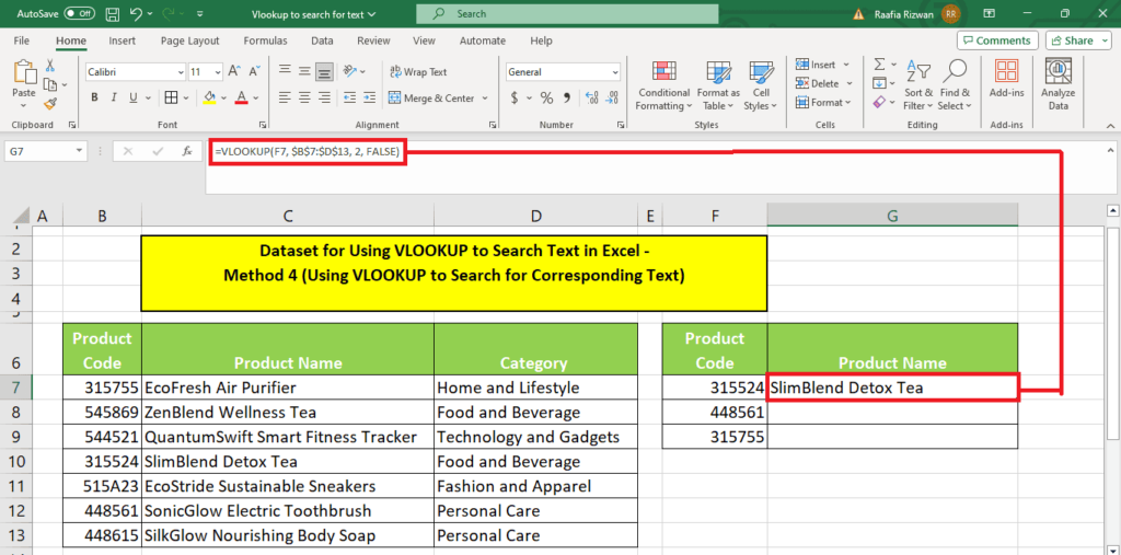
2. Drag the Fill Handle tool to input the formula in the remaining cells.
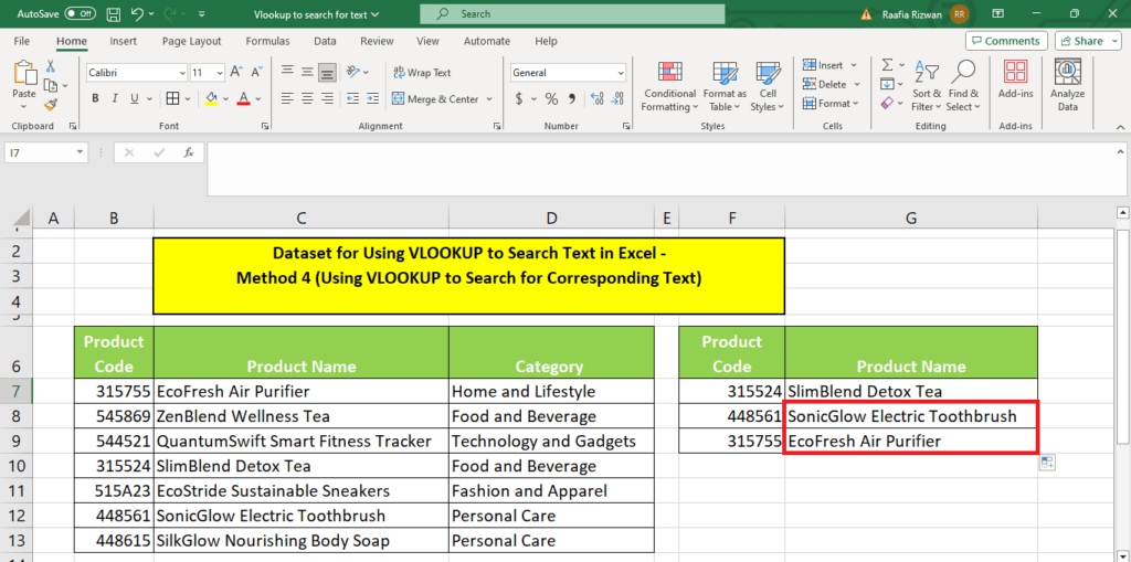
Note: Here, we've used the absolute cell reference using the $ sign ($B$7:$D$13) to keep it unchanged while dragging the Fill Handle to auto-fill the formula across the table.
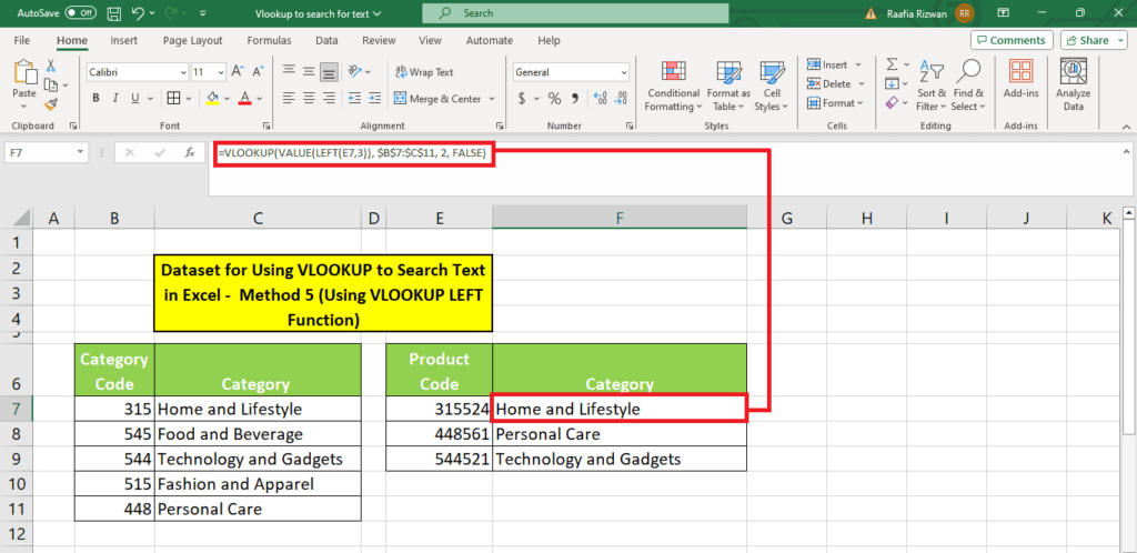
Method 5 – Using LEFT and RIGHT VLOOKUP functions to search for matching text
This method uses the VLOOKUP formula to search for text on the left and right in a dataset.
5.1 Combining LEFT and VLOOKUP to search for codes
Imagine that the starting 3 digits of the product code indicate the product category. Now, if we have a set of product codes, we can extract the product category using the LEFT function in the VLOOKUP formula.
1. Type this formula in your output table:
=VLOOKUP(VALUE(LEFT{Cell address of lookup value},{Number of digits}, {Dataset range with $ sign}, {Column index number}, {TRUE or FALSE})
=VLOOKUP(VALUE(LEFT(E7,3)), $B$7:$C$11, 2, FALSE)
Next, press Enter and drag the Fill Handle to auto-fill the formula across the table.
5.2 Combining RIGHT and VLOOKUP to search for codes
The store updates out-of-stock product codes with product code names + OOS.
In the product list, only 6-digit codes are allowed. The program automatically truncates the 3-digit product code on the left.
This means that a simple VLOOKUP formula cannot work.
Using the RIGHT VLOOKUP function, the inventory manager can quickly scan through the out-of-stock products.
1. Type this formula in your output table:
=VLOOKUP(RIGHT{Cell address of lookup value},{Number of digits}, {Dataset range with $ sign}, {Column index number}, {TRUE or FALSE})
=VLOOKUP(RIGHT(E7,6), $B$7:$C$13, 2, FALSE)
Hit Enter and use the Fill Handle to auto-fill the formula across the table:
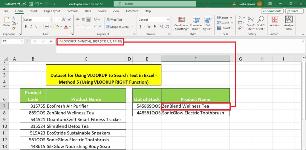
Note: If you're using the LEFT and RIGHT functions for a numeric lookup value, add VALUE with the lookup value like this: VALUE(RIGHT(E7,6)).
Wrapping up
We discussed five ways to use the VLOOKUP formula to search for text and numerical values in Excel. The easiest way is to enter the text in the formula. But Vlookup's functionalities extend beyond just the find function, which the rest of the methods cover.
Learn more about Excel with these helpful step-by-step guides:
- How to use VLOOKUP with COUNTIF
- How to sum all matches with VLOOKUP in Excel
- How to use VLOOKUP to find the last value in the column in Excel
About the Author