
Excel: Range lookup with VLOOKUP – 5 examples


Table of Contents
If you want to learn how range lookup with VLOOKUP works in Excel, you’ve come to the right place.
Using the VLOOKUP function in Microsoft Excel helps us find information in large tables quickly and accurately. One of the coolest features of VLOOKUP is its ability to look for a close match or the exact data you need, known as range lookup. This article is your friendly guide to understanding how this works. We'll show you step-by-step how to use the range lookup feature with VLOOKUP, complete with easy-to-follow examples.
Prime Day may have closed its doors, but that hasn't stopped great deals from landing on the web's biggest online retailer. Here are all the best last chance savings from this year's Prime event.
- Sapphire 11348-03-20G Pulse AMD Radeon™ RX 9070 XT Was $779 Now $719
- AMD Ryzen 7 7800X3D 8-Core, 16-Thread Desktop Processor Was $449 Now $341
- Skytech King 95 Gaming PC Desktop, Ryzen 7 9800X3D 4.7 GHz Was $2,899 Now $2,599
- LG 77-Inch Class OLED evo AI 4K C5 Series Smart TV Was $3,696 Now $2,996
- AOC Laptop Computer 16GB RAM 512GB SSD Was $360.99 Now $306.84
- Lexar 2TB NM1090 w/HeatSink SSD PCIe Gen5x4 NVMe M.2 Was $281.97 Now $214.98
- Apple Watch Series 10 GPS + Cellular 42mm case Smartwatch Was $499.99 Now $379.99
- AMD Ryzen 9 5950X 16-core, 32-thread unlocked desktop processor Was $3199.99 Now $279.99
- Garmin vívoactive 5, Health and Fitness GPS Smartwatch Was $299.99 Now $190
*Prices and savings subject to change. Click through to get the current prices.
So, without wasting another second, let’s dive in!
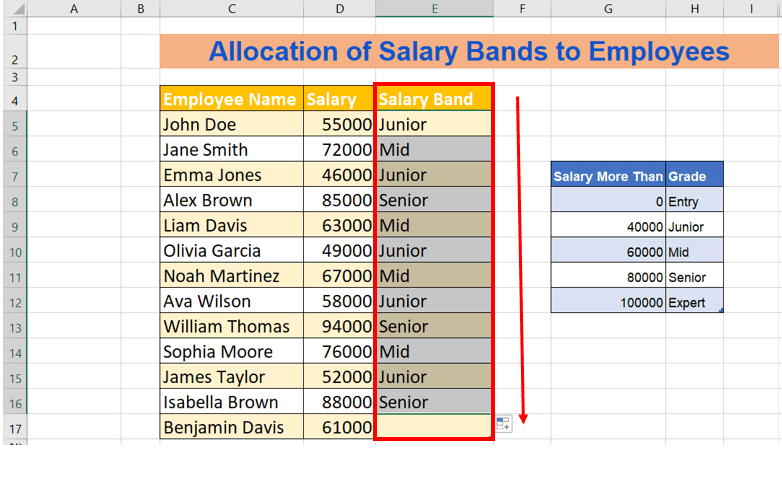
Example 1 – Allocation of salary bands to employees
In this example, employees are assigned a grade based on their salary. The grade is determined by the range in which their salary falls according to the Salary Bands Lookup Table.

We’ll explore how to allocate salary bands to a list of employees based on their earnings. The dataset provided here includes an example where employees’ salaries are matched against predefined salary bands to determine their respective grades.
The table to the right outlines the salary bands, indicating the minimum salary required to qualify for each grade, ranging from ‘Entry’ to ‘Expert’. We’ll use the VLOOKUP function to match each employee’s salary to these bands and assign the correct grade in Column E. The generic formula for the VLOOKUP function is:
=VLOOKUP(lookup_value, table_array, col_index_num, [range_lookup])
Here, the fourth argument ([range_lookup]) can be either TRUE (1) or FALSE (0). TRUE or 1 signifies that we are looking for an Approximate Match, which is what we need when dealing with salary ranges, as exact matches are unlikely. If this argument is omitted, VLOOKUP defaults to TRUE.
For our example, we would be using TRUE.
- Select Cell D5 and enter the formula:
=VLOOKUP(D5,$G$7:$H$12,2,TRUE) - After inserting the VLOOKUP formula, press Enter key to see the desired matched value which in our case is Junior for employee John Doe.
Note: The dollar signs ($) makes the reference absolute, which means if you copy the formula to another cell, the reference will stay the same. It will always look at the cells G7 to H12 for the table array.

- Drag the fill handle down from Cell E5 to fill the remaining cells in Column E with the VLOOKUP formula. All employees will now have their salary bands assigned, based on the salary band table.
Note: Keep in mind that the salary band table must be sorted in ascending order since VLOOKUP’s approximate match feature depends on this order to function correctly. If the table is not sorted correctly, the VLOOKUP function may return incorrect grades.
Example 2 – Determining fiscal quarters from dates with VLOOKUP
A fiscal quarter is a three-month period on a company’s financial calendar, and there are four such quarters in a fiscal year.
In this part of our guide, we will assign a fiscal quarter—Q1, Q2, Q3, or Q4—to a series of dates. This function helps us match each date to a corresponding quarter based on the defined date ranges.

- Click on cell C5 next to the first date (14-May-23)
- Type in the VLOOKUP formula:
=VLOOKUP(B5,$E$6:$F$9,2,TRUE)

- B5 is the lookup value, the cell that contains the date you want to evaluate.
- $E$6:$F$9 is the table array, the range of cells that contains your fiscal quarters’ data. The dollar signs indicate an absolute reference, which will not change as you copy the formula down.
- 2 is the index number, which tells VLOOKUP to return the value from the second column of the table array (the Quarter column).
- TRUE indicates that VLOOKUP should find an approximate match, which is what you need for date ranges.
- Press Enter, and Excel will display the fiscal quarter for the date in cell B5.

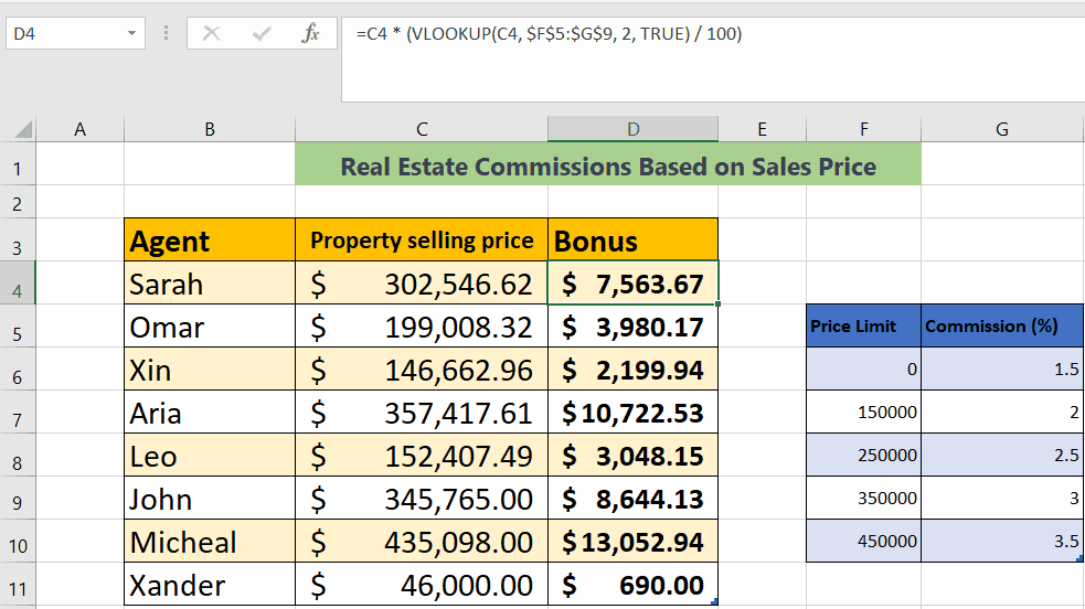
Method 3 – Calculating real estate commissions based on sales price with VLOOKUP
We will help you calculate the commission (bonus) each real estate agent earns based on the selling price of properties they’ve sold, using a tiered commission structure.
Our data is set up on two tables :
- The ‘Agent’ and ‘Property Selling Price’ are in columns B and C, respectively.
- The ‘Price Limit’ and ‘Commission (%)’ tables are placed in columns F and G.

- Click on cell D4 to determine the commission for the first agent (Sarah).
- Enter the VLOOKUP formula:
=VLOOKUP(C4, $F$5:$G$9, 2, TRUE)

- After entering the formula, multiply the result by Sarah’s selling price to get the actual commission amount:
=C4 * (VLOOKUP(C4, $F$5:$G$9, 2, TRUE) / 100)

- Press Enter and then drag down from the first cell to the last on the column.
Example 4 – Assigning employee performance ratings using VLOOKUP
The dataset includes two parts; a list of employees with their quarterly scores and a rating table with score ranges. Column B shows employee names, and Column C has their scores. In another section, Columns F and G match scores with letter grades from ‘F’ to ‘A+’. We’ll use this data to give each employee a grade based on their score. We will use VLOOKUP to evaluate the performance ratings.

- Select Cell D4 next to the first employee’s name.
- Enter the VLOOKUP formula:
=VLOOKUP(C4, $F$5:$G$11, 2, TRUE)

- Press Enter. Excel will display Anna’s performance rating based on her quarterly review score.
- Move your cursor to the lower-right corner of Cell D4 until it turns into a plus sign (the fill handle).
- Click and drag the fill handle down through Cell D12 to copy the formula to the other cells in Column D.
- The performance ratings for all employees listed will now be displayed at once based on their review scores.

Note: The scores in your lookup table (Column F) must be sorted in ascending order for the VLOOKUP function to correctly perform an approximate match. If the scores are not in order, the function may return incorrect ratings.
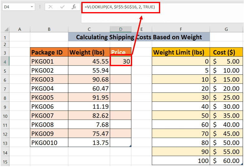
Example 5 – Calculating shipping costs based on weight with VLOOKUP
The dataset includes two tables: one with 10 packages listed by ID and weight, and a second table with weight limits and corresponding shipping costs. The objective is to determine the shipping price for each package based on its weight using Excel’s VLOOKUP function.

- Click on cell D4, where the price for the first package will be calculated.
- Insert the following VLOOKUP formula to calculate the price of the package according to the weight :
=VLOOKUP(C4, $F$5:$G$16, 2, TRUE)
- Press Enter and it will autofill the price column OR drag from the corner of the cell D4 till the end of the table.

Tip: In order to get the $ sign for price in the Price column, you can choose the column and then the $ option from the home tab ribbon under the Number section.

Conclusion
With the examples provided in this tutorial, you should now be equipped to effectively utilize the range lookup capabilities of VLOOKUP in your Excel spreadsheets. To learn more about how the VLOOKUP function works in Excel, give these helpful guides a read:
- How to use VLOOKUP with COUNTIF in Excel
- How to use VLOOKUP to find the last value in the column in Excel
- How to sum all matches with VLOOKUP in Excel
About the Author