How to combine cells in Excel – Bring information together in one cell

Table of Contents
It can be a little daunting looking at spreadsheet after spreadsheet of information in a Microsoft Excel workbook. Page after page of names, addresses, wages, inventory, and more can be a lot to manage. Thank goodness for Microsoft Excel Formula.
Every formula represents a handy shortcut for users, which in turn makes spreadsheets and workbooks more efficient are clearer. Having information laid out and clear to see is one thing, but combining said information for the sake of easy-to-find information and clearer charts is a handy feature.
Prime Day is finally here! Find all the biggest tech and PC deals below.
- Sapphire 11348-03-20G Pulse AMD Radeon™ RX 9070 XT Was $779 Now $739
- AMD Ryzen 7 7800X3D 8-Core, 16-Thread Desktop Processor Was $449 Now $341
- ASUS RTX™ 5060 OC Edition Graphics Card Was $379 Now $339
- LG 77-Inch Class OLED evo AI 4K C5 Series Smart TV Was $3,696 Now $2,796
- Intel® Core™ i7-14700K New Gaming Desktop Was $320.99 Now $274
- Lexar 2TB NM1090 w/HeatSink SSD PCIe Gen5x4 NVMe M.2 Was $281.97 Now $214.98
- Apple Watch Series 10 GPS + Cellular 42mm case Smartwatch Was $499.99 Now $379.99
- ASUS ROG Strix G16 (2025) 16" FHD, RTX 5060 gaming laptop Was $1,499.99 Now $1,274.99
- Apple iPad mini (A17 Pro): Apple Intelligence Was $499.99 Now $379.99
*Prices and savings subject to change. Click through to get the current prices.
How to combine cells in Excel
Rather than just talking about it, let's show how to do it. There are actually two formulae when considering how to combine cells in Excel using the Ampersand symbol (&) and the CONCAT function. Essentially, the Ampersand function is great for combining two cells, with CONCAT being a preferred function for multiple combined cells. Let's go through both functions and how to implement them:
Ampersand – How to combine cells in Excel
The following is for combining just two cells, to combine information from more cells, please skip to the next step below. Let's start by clicking into the cell where the formula result needs to lie. From here we need to tell Excel that formula is about to be entered by typing = followed by the first cell reference. This should then be followed by an Ampersand and a space enclosed in quotation marks, followed by another Ampersand and the second cell reference.
As we can see from the below example, the formula would be =A2&” “&D2.
Finally, if the whole column needs to display this formula, left-click on the bottom-right corner and drag the cell box down to apply the formula to the whole column as displayed below.
CONCAT – How to combine cells in Excel
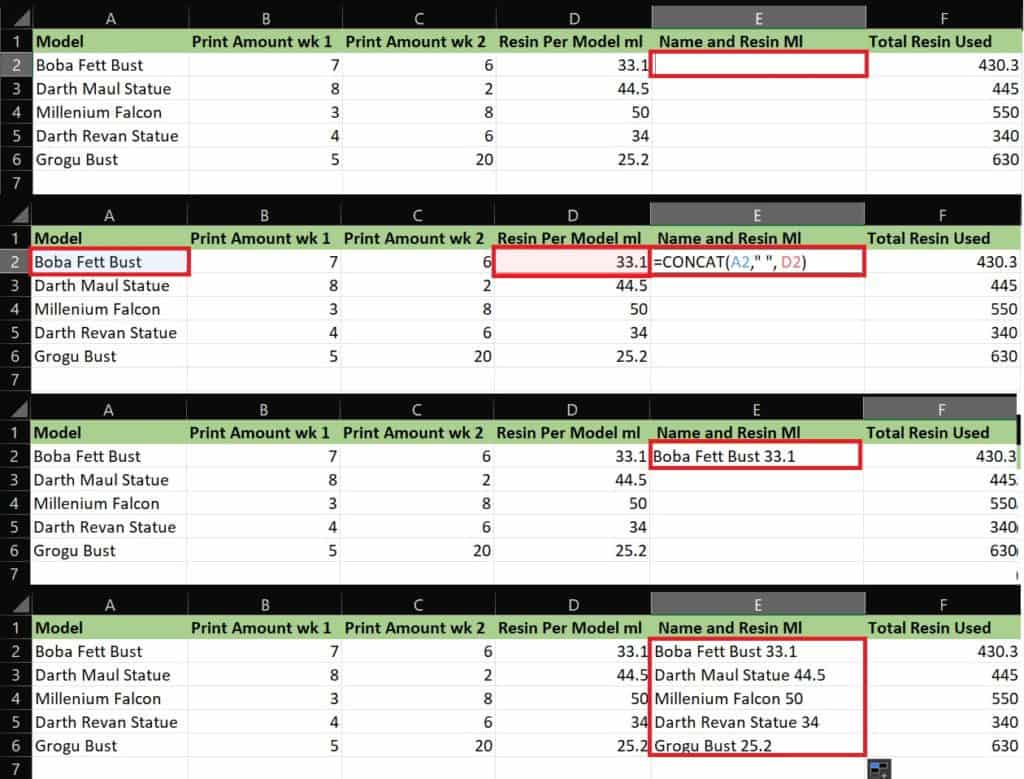
This formula is applied in the same way as the Ampersand formula above, only it supports multiple cell inputs, meaning multiple combinations of cells. Click into the cell where the combination needs to lie and start things off with a = symbol to initiate a formula input. Next, write CONCAT followed by a bracket and cells references needed. The cell references need commas in between and the space wrapped in quotation marks to put a space after every comma. Once inputted, close the formula off with a closing bracket.
The example we've used below reads as =CONCAT(A2,” “,D2).
Again, if the spreadsheet needs the formula result copied to the whole column, left-click the bottom right corner of the CONCAT cell and drag over any cells needed in the same column.
Thanks for choosing PC Guide for help learning how to combine cells in Excel. For more help with Excel and Microsoft Office, please visit and bookmark our Office hub.


