How to freeze a row in Excel – Keep track of long spreadsheets

Table of Contents
It can be a challenge keeping track of large amounts of information in Microsoft Excel, but there's also a robust toolset to help make navigating daunting spreadsheets and workbooks easier. This is why Microsoft Excel is the go-to spreadsheet software and has been for years.
Not only is Microsoft Excel full of formulae and features that make users’ lives easier, spreadsheets are exportable to suit a range of software packages. This comes in super handy when it comes down to any form of business management and more.
Prime Day is finally here! Find all the biggest tech and PC deals below.
- Sapphire 11348-03-20G Pulse AMD Radeon™ RX 9070 XT Was $779 Now $739
- AMD Ryzen 7 7800X3D 8-Core, 16-Thread Desktop Processor Was $449 Now $341
- ASUS RTX™ 5060 OC Edition Graphics Card Was $379 Now $339
- LG 77-Inch Class OLED evo AI 4K C5 Series Smart TV Was $3,696 Now $2,796
- Intel® Core™ i7-14700K New Gaming Desktop Was $320.99 Now $274
- Lexar 2TB NM1090 w/HeatSink SSD PCIe Gen5x4 NVMe M.2 Was $281.97 Now $214.98
- Apple Watch Series 10 GPS + Cellular 42mm case Smartwatch Was $499.99 Now $379.99
- ASUS ROG Strix G16 (2025) 16" FHD, RTX 5060 gaming laptop Was $1,499.99 Now $1,274.99
- Apple iPad mini (A17 Pro): Apple Intelligence Was $499.99 Now $379.99
*Prices and savings subject to change. Click through to get the current prices.
How to freeze a row in Excel

What do we mean by how to freeze a row in Excel? Well, there are a few ways to do it, but we're going to concentrate on the two most useful methods. Learning how to freeze a row in Excel allows for collum headers to follow scrolls down a long spreadsheet, for example. It also comes in handy for keeping figures in view no matter where users are on a specific spreadsheet.
Let's have a look at how to freeze a row in Excel. More specifically freezing top rows and panes:
Freeze Top Row – How to freeze a row in Excel
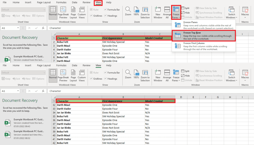
Freeze Top Row comes in really handy for users looking to keep column headings or a top row of information with the reader when scrolling through an Excel spreadsheet. Not only is it handy to have information in front of users at all times, but it adds to the presentation and professionalism of a workbook.
Start by hitting the View tab on the Excel top ribbon and going to the ‘Freeze Panes' button. From the dropdown, select ‘Freeze Top Row'. In our example above, column headers will follow a user's scroll to make navigation of this certain spreadsheet as easy as possible. Want to turn this feature off? Just click the Freeze Top Row button again to disable it.
Freeze Panes – How to freeze a row in Excel
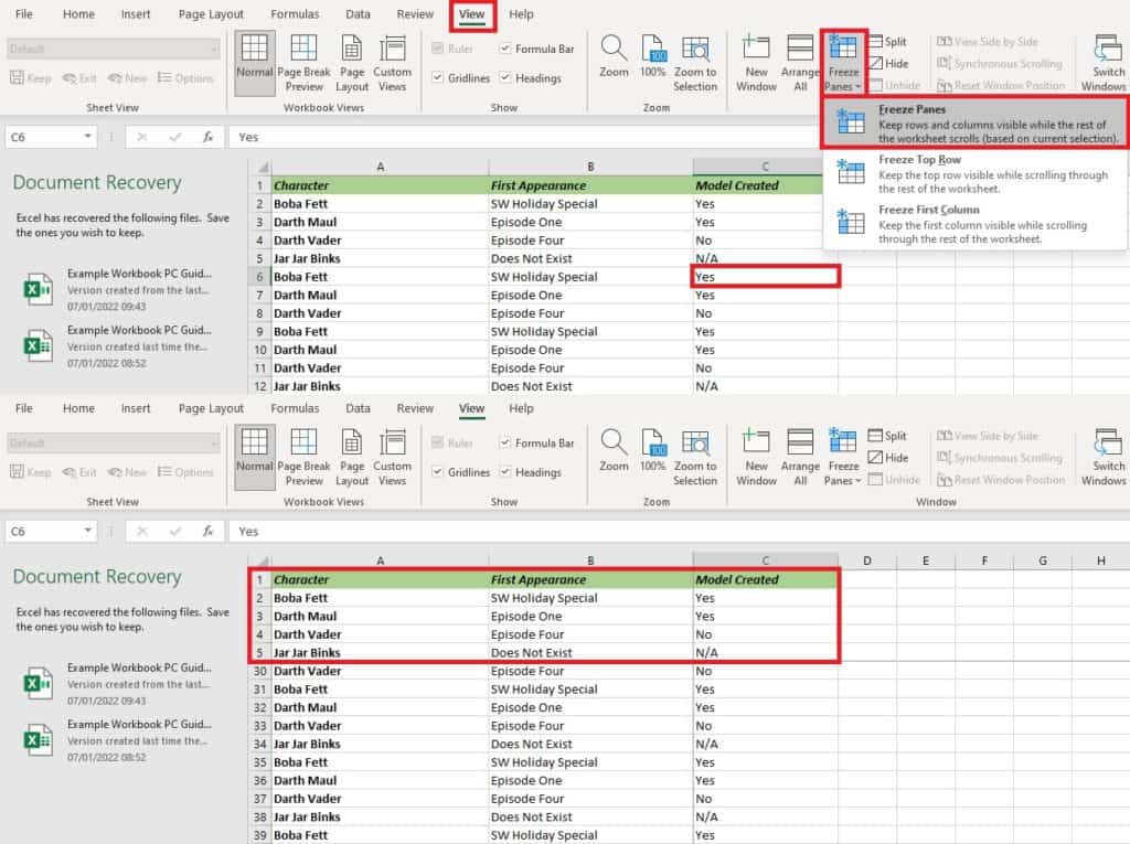
Freeze Panes allows users to select as many cells as they'd like in a block to freeze and follow a user’s scroll throughout a document. Perhaps there's a set of figures that need to be followed and checked against the rest of the spreadsheet? This feature ensures Excel users can do just that.
To start, select a cell that is at the right-hand corner of the selection area as shown above. Then go to the View tab in the Excel ribbon and hit ‘Freeze Panes, selecting ‘Freeze Panes' from the dropdown menu.
As seen in the example above, the selected cells will now follow a user’s scroll. Simply click the option again to turn it off if desired.
Thanks for choosing PC Guide for learning how to freeze a row in Excel. Users may want to try the ‘Freeze First Column' option too, but we found that the options covered above provide all the functionality necessary to get ahead.
For more helpful how-to guides on Excel or Microsoft Office, please visit and bookmark our Office hub.


