How to use COUNTIF function in Excel – 8 examples

Table of Contents
Wondering how to use COUNTIF in Excel? We’ve got you covered.
Excel has many functions you can use in different scenarios. These functions can prove to be extremely useful in several situations, especially when dealing with a large data set. One of the functions is COUNTIF, which can help speed up the work. However, using it can seem confusing at first, especially if you’re new to the software.
Prime Day is finally here! Find all the biggest tech and PC deals below.
- Sapphire 11348-03-20G Pulse AMD Radeon™ RX 9070 XT Was $779 Now $739
- AMD Ryzen 7 7800X3D 8-Core, 16-Thread Desktop Processor Was $449 Now $341
- ASUS RTX™ 5060 OC Edition Graphics Card Was $379 Now $339
- LG 77-Inch Class OLED evo AI 4K C5 Series Smart TV Was $3,696 Now $2,796
- Intel® Core™ i7-14700K New Gaming Desktop Was $320.99 Now $274
- Lexar 2TB NM1090 w/HeatSink SSD PCIe Gen5x4 NVMe M.2 Was $281.97 Now $214.98
- Apple Watch Series 10 GPS + Cellular 42mm case Smartwatch Was $499.99 Now $379.99
- ASUS ROG Strix G16 (2025) 16" FHD, RTX 5060 gaming laptop Was $1,499.99 Now $1,274.99
- Apple iPad mini (A17 Pro): Apple Intelligence Was $499.99 Now $379.99
*Prices and savings subject to change. Click through to get the current prices.
In this guide, we’ll explain how to use the COUNTIF function in Excel so you can finish your work quickly.
How to use COUNTIF in Excel
Scenario on hand: We have a dataset of student's marks.
What we want to accomplish: Explore how to use the COUNTIF function in Excel in the following ways:
- Simple mathematical criteria
- Simple mathematical criteria with cell reference
- Multiple mathematical criteria
- Exact match
- Partial match
- OR criteria
- Count blanks
- Count duplicates
Simple mathematical criteria
The COUNTIF function is quite simple because it only requires a range and criteria. In our dataset, we have 9 student names and the marks they obtained throughout a course. We want to count the number of students who qualify a grade criteria.
To do this, we define the criteria first:

The next step is entering the formula. Here's the syntax of the COUNTIF function in Excel:
=COUNTIF(range, criteria)
For our case, here's what the formula looks like:
=COUNTIF($I$6:$I$14,K6)
Note that we add $ to the range to make the formula dynamic. We input this formula in the first cell, then drag it using the small square at the bottom called the ‘Fill Handle Tool.'
Here are the results:

In this example, we have used the ‘lesser than' and ‘greater than' criteria. However, we have summarized all the simple mathematical criteria for you in a tabular form so you can refer to it while using the COUNTIF function in Excel:
| Criteria | Formula Example | Description |
| Count if equal to | =COUNTIF(B3:B16,”=90%”) | Count cells where the value is equal to 90%. |
| Count if less than | =COUNTIF(B3:B16,”<90%”) | Count cells where the value is less than 90% |
| Count if greater than | =COUNTIF(B3:B16,”>90%”) | Count cells where the value is greater than 90% |
| Count if less than or equal to | =COUNTIF(B3:B16,”<=90%”) | Count cells where the value is less than or equal to 90%. |
| Count if greater than or equal to | =COUNTIF(B3:B16,”>=90%”) | Count cells where the value is greater than or equal to 90%. |
| Count if not equal to | =COUNTIF(A2:A10,”<>90%”) | Count cells where the value is not equal to 90%. |
Simple mathematical criteria with cell reference
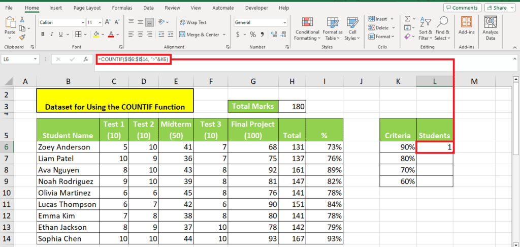
In the above method, we added the > and < signs in the cell reference. We repeat the same example, but without the > and < signs in the cell reference:

To calculate the number of students below the defined criteria, here's the formula we use:
=COUNTIF({range},”>”&{cell reference})
For our dataset, the formula looks like this:
=COUNTIF($I$6:$I$14, “>”&K6)
Here's the result:

Expanding the formula using the Fill Handle Tool, we get:

Multiple mathematical criteria
In the first method, we found how to use the COUNTIF function to count the number of entries with simple mathematical criteria. The use of this function shows that all 9 students have secured above 60% and 70% marks.
In this method, we introduce grades to the criteria like this:

To calculate the grade each student has secured, we have to use the following COUNTIF formula:
=COUNTIF(range,”criteria 1″)-COUNTIF(range,”criteria 2″)
=COUNTIF($I$6:$I$14,L7) – COUNTIF($I$6:$I$14,L6)
Here are the results:

Exact match
In this method, we want to see how many times students secured 10/10 marks on their tests.
Here's the formula we use for this:
=COUNTIF(C6:F14,”10″)
Upon pressing enter, we see that on 8 instances, students have secured 10/10 marks on their tests throughout the course:

Partial match
In our dataset, we want to count student names that have “son” in them. To do this, we modify the formula a bit with wildcard characters like this:
=COUNTIF(range, “*{phrase}*”)
Here's what it looks like for our dataset:

We get a count of three names with the letters “son” in them.
OR criteria
If you want to count cells that have either one value or the other, the OR criteria is the way to go.
The OR criteria is nothing but a + in between two COUNTIF functions.
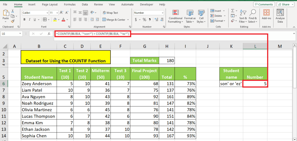
In our dataset, we want to find names of students partially matching “son” or “ez.” Here's the formula we use for it and the result:
=COUNTIF(B6:B14, “*son*”) + COUNTIF(B6:B14, “*ez*”)

Count blanks
In Excel, you can even use the COUNTIF function to count the blanks in your data set. For this example, we have modified the data to show two blank cells. We then input the following formula to count the blank and non-blank cells:
- Blank cells (all data types): COUNTIF({range},””)
- Blank cells (text): COUNTIF(range,”<>”&”*”)
- Non-blank cells: COUNTIF({range},”<>”&””)
Here's the output when we use formulas 1 and 3 to calculate blank and non-blank cells:

Count Duplicates
You can even use the COUNTIF function to calculate duplicates in your dataset. A simple loop formula using COUNTIF is required for this:
=COUNTIF({table range}, {value})>1
In our dataset, we want to see whether the students scored the same marks they did in their first assessment.
Here's the formula we use:
=COUNTIF(C6:G6,C6)>1

Using the Fill Handle Tool, we expand the formula and see that four students have secured the same marks in two or all three of their tests:

Wrapping up
And that's how you can use the COUNTIF function in Excel. Clearly, this function is handy because it saves you a lot of time going through your results and counting them individually. Instead, let Excel do all the hard work for you by using this function following the steps above.
Learn more about Excel and how it works through these guides:

