How to use VLOOKUP to find approximate text match in Excel - 4 methods

You can trust PC Guide: Our team of experts use a combination of independent consumer research, in-depth testing where appropriate - which will be flagged as such, and market analysis when recommending products, software and services. Find out how we test here.

If you want to learn how to use VLOOKUP to find approximate text match in Excel, you’ve come to the right place.

VLOOKUP’s syntax includes a True and False argument. While False returns an exact match, True looks for an approximate match. However, the True argument isn’t very efficient for text matches. Today, we explore alternative ways you can use VLOOKUP to find an approximate text match in your dataset.

So, without any further ado, let’s dive in!

How you can use VLOOKUP to find an approximate text match in Excel

Scenario on hand: We have a fictional dataset of Hollywood movie names with their year of release, name, male lead name, female lead name, and IMDB rating.

What we want to accomplish: We want to understand how to use VLOOKUP to find an approximate match for text in Excel. We will explore four methods for this:

Using wildcards to return a cell that begins with a particular text
Using wildcards to return a cell that ends with a particular text
Using wildcards to return a cell that contains particular text
Using a helper column to return a cell with two corresponding values

Method 1: Using wildcards to return a cell that begins with a particular text

Wildcards are a great way to fetch partial text matches. In this first method, we will use wildcards to return movie names that start with a particular text.

Here’s the formula you can use to fetch any cell that begins with a particular text value:

=VLOOKUP({Partial lookup value}&”*”,{Table array}, {Column index number}, FALSE)

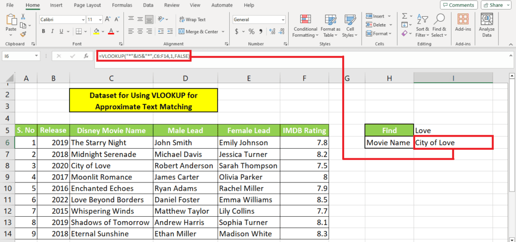
We applied this formula to search for a movie name that began with “Love”:

=VLOOKUP(I5&”*”, C6:F14,1, FALSE)

Here, we have the lookup text “Love” on I5. The wildcard &”*” after I5 signifies that the partial text will be at the beginning.

After entering the formula, here’s what we get:

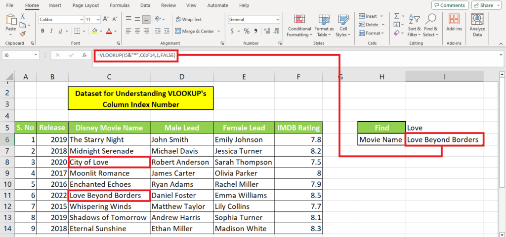
Learn how to create a spreadsheet in Excel using VLOOKUP for an approximate text match.

We have “Love” in two movie names. But since we used the wildcard symbol &”*” after the cell address of the lookup value, the formula fetches the movie with “Love” in the beginning.

Note: This formula can also be used to fetch partial words. For instance, “Love” could also fetch film titles with “Lovely,” “Lover,” or “Lovestruck.”

However, if multiple partial matches are found, the formula will return the first match rather than all matches.

Method 2: Using wildcards to return a cell that ends with a particular text

In the first method, we saw how we can use the wildcard symbols to fetch a cell value, which begins with the lookup text value. Let’s modify this formula to fetch the movie name that ends with the particular text.

Here’s the modified formula:

=VLOOKUP(“*”&{Partial lookup value}, {Table array}, {Column index number}, FALSE)

We applied this formula to our movie dataset this way:

=VLOOKUP(“*”&I5, C6:F14,1, FALSE)

We kept the lookup value the same. This time, the modified formula returned the movie that ends with “Love.” Here’s the formula in action:

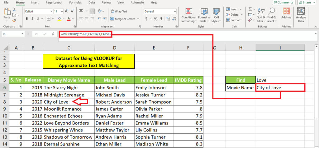
Note: This formula will not return movie names with anything after “Love.” So any movies with “Lovely,” “Lovestruck”, or “Loved” at the end will not be fetched.

However, it can fetch values like “clove”.

Although this formula uses “False” for an exact match, it is not case-sensitive. Here’s the result of this formula when we use “Love” in lowercase:

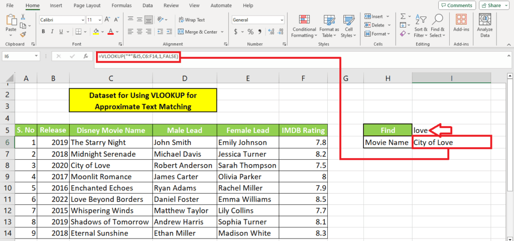
Learn how to create a table in Excel using the VLOOKUP function for approximate text match.

The result is the same when we enter the lookup value in uppercase:

Learn how to create a spreadsheet in Excel, including utilizing the VLOOKUP function for an approximate text match.

Method 3: Using wildcards to return a cell that contains particular text

If you are unsure whether the text you want to search for lies in the beginning or end, you can use the wildcards to search for a cell that contains the lookup value.

You can also use this formula if you are sure that your desired cell value contains a certain phrase:

=VLOOKUP(“*”&{Partial lookup value}&”*”, {Table array}, {Column index number}, FALSE)

Note that we have inserted the wildcard symbols & and “*” on both ends. This fetches cell values containing the phrase, whether in between, in the beginning, or at the end.

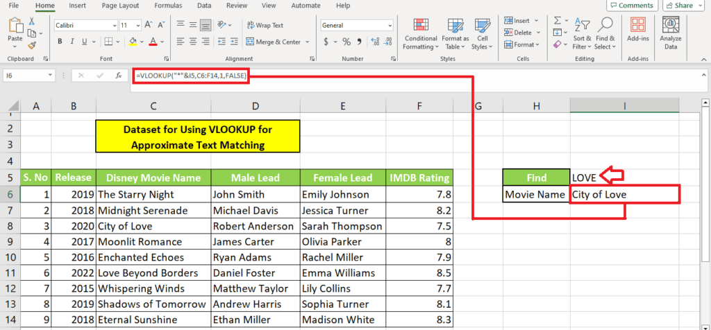
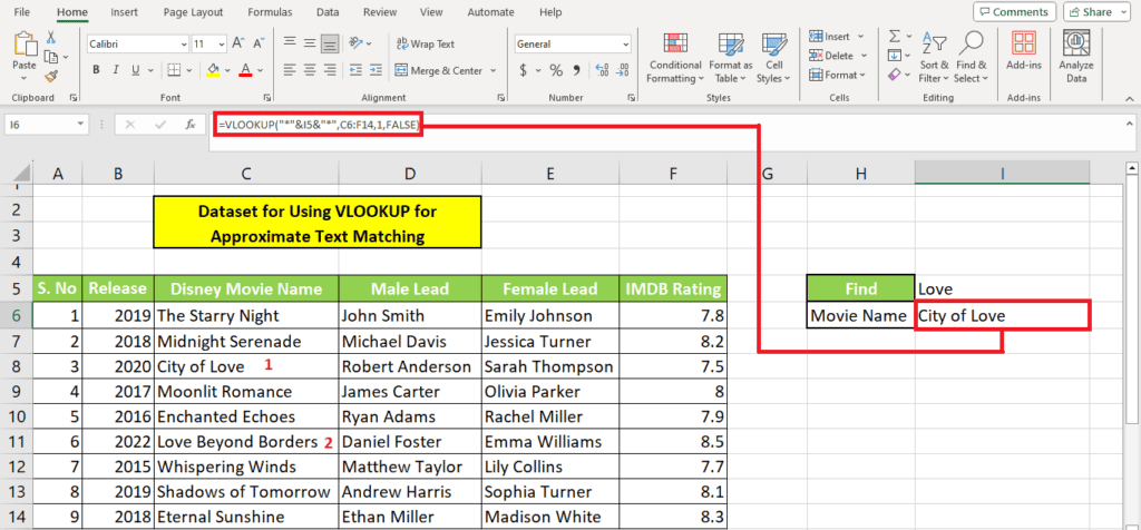
We applied this formula for our lookup value “love” again:

=VLOOKUP(“*”&I5&”*”, C6:F14,1, FALSE)

The formula fetched the first movie title that contains the phrase “love”:

Learn how to create a spreadsheet in Excel and use VLOOKUP for an approximate text match.

Instead of just returning the movie name or the first column, you can also enter a different column index number to get the corresponding value.

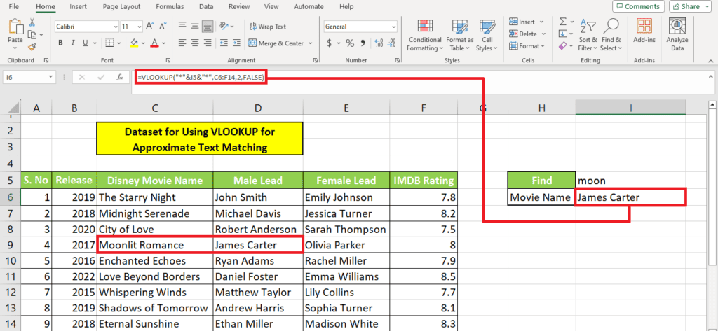
We used this formula to fetch the Actor name of a movie containing the phrase “moon”:

=VLOOKUP(“*”&I5&”*”, C6:F14, 2, FALSE)

Here’s the formula in action:

Method 4: Using a helper column to return a cell with two corresponding values

Wildcard symbols can be quite helpful in fetching the first value occurrence in a table. However, if you want to get a value that corresponds with another value and is not necessarily the first instance in the table, you can use a helper column.

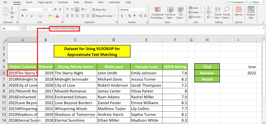
In the same dataset, add a helper column to the left.

Why add the helper column?

We add the helper column to the left since VLOOKUP searches for values from left to right and in the first column.

With this helper column, we can search for a movie name that matches values across two columns.

If we search for “love” using the “contains type” wildcard function, we get the first occurrence of love in the data:

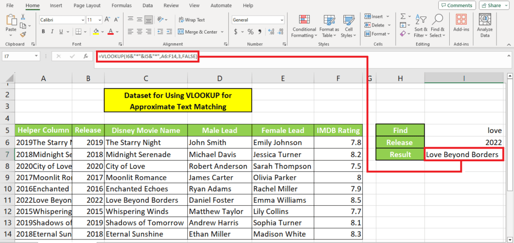
Learn how to create a spreadsheet in Excel with the use of approximate text match and VLOOKUP function.

But if we want to fetch a movie with “love” that was released in 2022, we add the helper column where we concatenate the values of the two columns.

Here’s the concatenate formula:

=CONCATENATE({Value 1}, {Value 2})

We used this formula to concatenate the release year and movie names in a single column:

=CONCATENATE(B6, C6)

Here’s how it worked out:

A screenshot of an Excel table with VLOOKUP functionality for approximate text matching.

Then, using a slightly modified VLOOKUP wildcard formula, we searched for a movie containing “love” released in 2022.

Here’s the formula:

=VLOOKUP({Lookup value in the beginning}&”*”&{Partial lookup value}&”*”, {Table array}, {Column index number}, FALSE))

We added the release year in the beginning and used this formula:

=VLOOKUP(I6&”*”&I5&”*”, A6:F14, 3, FALSE)

Here’s what the formula resulted:

Learn how to create a spreadsheet in Excel, utilizing the VLOOKUP function for an approximate text match.

Wrapping up

This was how to use VLOOKUP to find approximate text match in Excel. VLOOKUP can be used with wildcards to search for partial text in your data, either at the beginning or end. This formula is also helpful for searching for cells that contain the lookup phrase. Wildcards and VLOOKUP can also be used to search for data across two columns using a helper column. We demonstrated four examples where we searched for approximate text. You can also use these methods to search for partial text in your dataset.

Learn more about the VLOOKUP function through these helpful guides: