You can trust PC Guide: Our team of experts use a combination of independent consumer research, in-depth testing where appropriate - which will be flagged as such, and market analysis when recommending products, software and services. Find out how we test here.

If you want to see some examples of VLOOKUP with multiple IF conditions in Excel, you’ve landed on the right page.

Learning about the VLOOKUP and IF functions is extremely important if you want to master Excel. By combining these two functions, you can perform different tasks, which can help you greatly when dealing with large data sheets.

In this guide, we will share some examples of VLOOKUP with multiple IF conditions in Excel.

7 examples of IF conditions with VLOOKUP

Scenario on hand: We have a fictional dataset of noodles sales in a superstore. The superstore will make some inventory restocking and discounting decisions based on the analysis we conduct.

What we want to accomplish: We want to use IF conditions with VLOOKUP to:

Assign a value based on a number in the IF condition
Assign a value based on a cutoff in the IF condition
Calculate the discount price based on the remaining inventory
Search for products in the list
Search for a value across two tables
Using VLOOKUP to fetch values from two tables
Use 3 VLOOKUP in 1 IF condition

Condition 1 – Assign a value based on a number in the IF condition

Our fictional superstore stocks 3 brands of noodles with 3 flavors each. At the beginning of the month, they stock up their inventory and enter the inventory figure in the data.

At the end of the month, they revisit the inventory numbers to get an idea about sales.

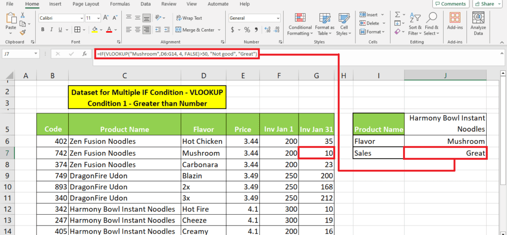
Here’s the defined criteria: If there are less than 50pcs of a certain brand’s flavor left in inventory, it means that the sales were great.

We use the following formula to get to this:

=IF(VLOOKUP(“{Lookup value}”,{Table array}, {Column index number}, FALSE)>{Cut off number}, “{Value if true}”, “{Value if false}”)

=IF(VLOOKUP(“Mushroom”,D6:G14, 4, FALSE)>50, “Not good”, “Great”)

Since the stock of the Mushroom flavor was not 10, which is not greater than 50, the formula returned “Great” as the value:

Condition 2 – Assign a value based on a cutoff in the IF condition

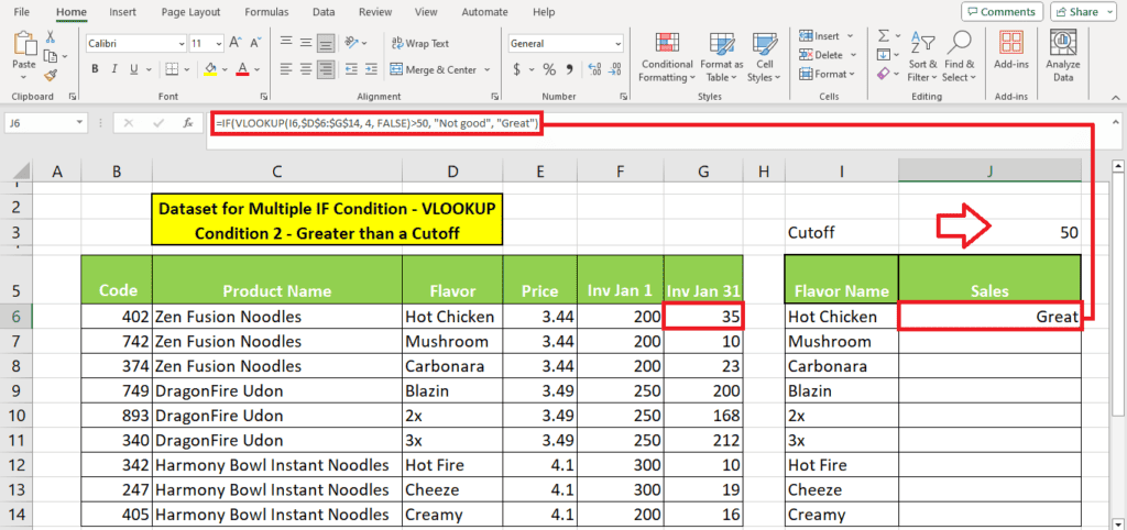
Alternatively, you can write the cutoff condition in a cell and reference it in the formula.

Here’s the formula you can use:

=IF(VLOOKUP({Cell reference of lookup value},,{Table array}, {Column index number}, FALSE)>{Cell address of cut off number}, “{Value if true}”, “{Value if false}”)

=IF(VLOOKUP(I6,$D$6:$G$14, 4, FALSE)>J3, “Not good”, “Great”)

You can also make a table to determine the sales condition of the different products like this:

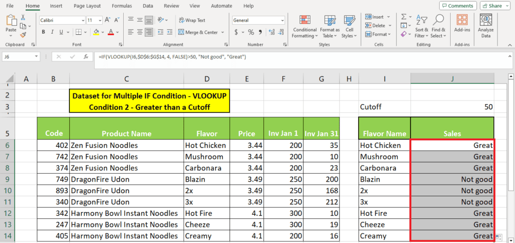
Note a small green square at the bottom right of the cell. This is the Fill Handle Tool.

Drag it downward to auto-fill the rest of the columns like this:

Condition 3 – Calculating the discount price based on the remaining inventory

You can easily calculate a discounted price based on a calculation formula. However, if you wish to apply a condition to the discounts, you will need to use VLOOKUP and IF together.

In this case, the superstore wishes to apply a 20% discount on the products only if the remaining inventory exceeds 50 pieces.

Here’s the formula for that:

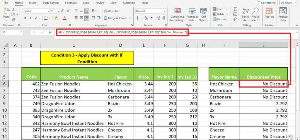
=IF(VLOOKUP(“{Product Name}”,{Table array},{Column index number to lookup},FALSE)>{Cut off number},VLOOKUP(“Product Name”,{Table array},{Column index number to apply discount},FALSE)*{Discount %},”No Discount”)

=IF(VLOOKUP(“Hot Chicken”,D6:G14,4,FALSE)>50,VLOOKUP(“Hot Chicken”,D6:G14,2,FALSE)*80%,”No Discount”)

Upon pressing Enter, we get the following result:

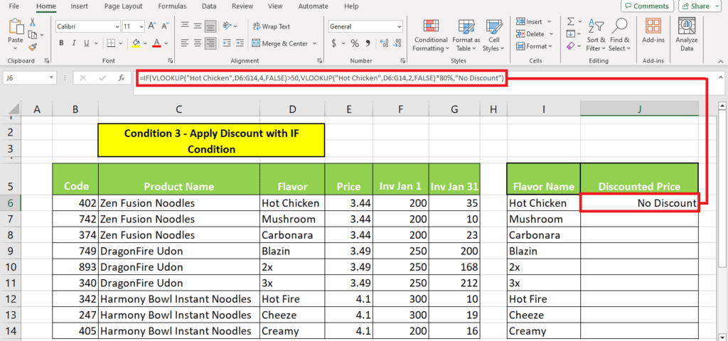
No discount is applicable since the Hot chicken flavor’s inventory is less than 50.

We cannot drag the fill handle tool to auto-fill the other rows on the table. For that, we need a slight modification in the formula:

Add the cell address instead of the product name in the formula.
Add a $ sign to add an absolute reference.

Note: We add the $ sign to only the table array so the formula doesn’t automatically shift the numbers down. We don’t add the $ to the cell address of the product since it needs to change to calculate the discounted price for different products.

Here’s the modified formula you need to add if you wish to use the Fill Handle tool to auto-complete other entries:

=IF(VLOOKUP(“{Cell Address for Product Name}”,{Table array with $},{Column index number to lookup},FALSE)>{Cut off number},VLOOKUP(“Cell Address for Product Name”,{Table array with $},{Column index number to apply discount},FALSE)*{Discount %},”No Discount”)

=IF(VLOOKUP(I6,$D$6:$G$14,4,FALSE)>50,VLOOKUP(I6,$D$6:$G$14,2,FALSE)*80%,”No Discount”)

Here’s the formula in action:

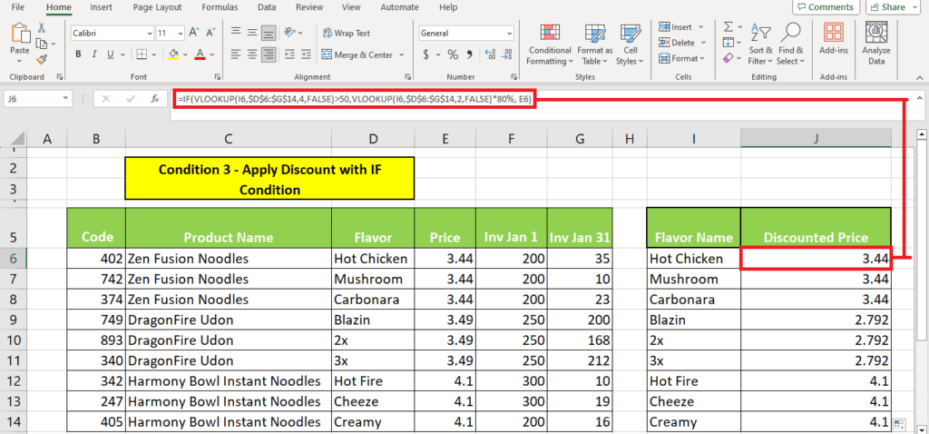
Another change in the formula can give us the original price instead of “No Discount” in the new table.

Instead of “No Discount”, you can add the cell reference of the price from the original table.

Here’s how we modified this formula:

=IF(VLOOKUP(I6,$D$6:$G$14,4,FALSE)>50,VLOOKUP(I6,$D$6:$G$14,2,FALSE)*80%,E6)

Here’s the resultant table:

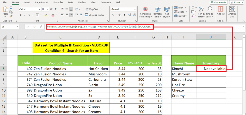
Condition 4 – Searching for products in the list

VLOOKUP can be used to search for customer’s requested products in the product dataset.

If the product is not found in the table, the formula returns “Not available”.

Here’s the formula for applying this condition:

=IF(ISNA(VLOOKUP({Cell address of the lookup value},{Table array with $},{Column index number to return the value},FALSE)),”Not available”,VLOOKUP({Cell address of the lookup value},{Table array with $},{Column index number to return the value},FALSE))

=IF(ISNA(VLOOKUP(I6,$D$6:$G$14,4,FALSE)),”Not available”,VLOOKUP(I6,$D$6:$G$14,4,FALSE))

Here’s what we get when we search for a product not available in the list:

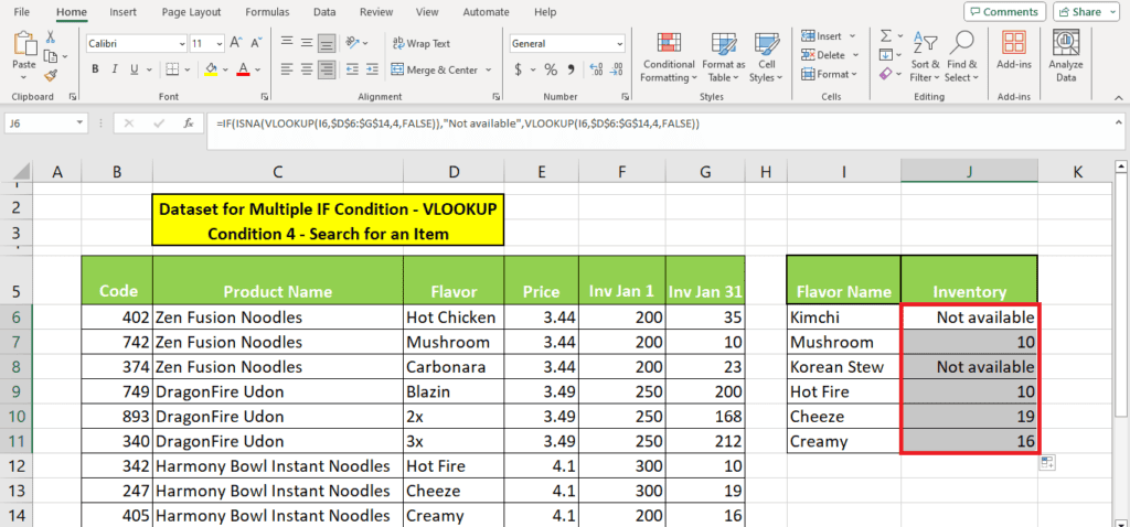
We expand the formula across the table using the Fill Handle tool:

Condition 5 – Searching for a value across two tables

You can search for a value across two tables using VLOOKUP and IF combined.

Following the same example, we now have two tables for January and February where the prices of the products are changed.

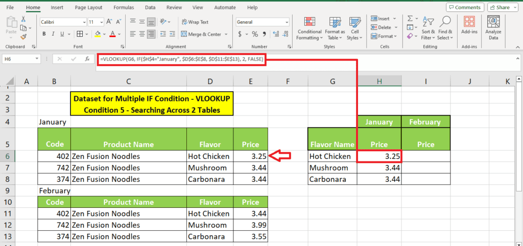
We have a separate table to compare the prices across the two months. To fetch the value from the different tables, here’s the formula:

=VLOOKUP({Cell address of product name}, IF({Cell with lookup value with $}=”{Lookup value}”, {Table array to fetch value if cell with lookup value matches lookup value} {Table array to fetch value if cell with lookup value does not match lookup value} ), {Column index number to fetch value}, FALSE)

=VLOOKUP(G6, IF($H$4=”January”, $D$6:$E$8, $D$11:$E$13), 2, FALSE)

We see that since the cell matched January, we get the price values from the January table array $D$6:$E$8:

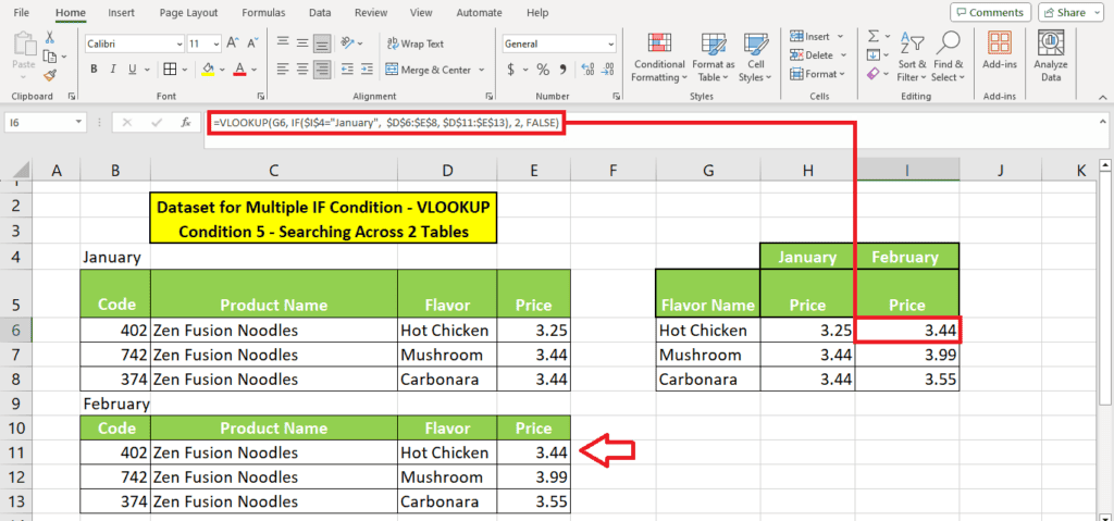
For fetching February values, we just switch the order of the table arrays in the formula:

=VLOOKUP(G6, IF($I$4=”January”, $D$6:$E$8, $D$11:$E$13), 2, FALSE)

Since “February” does not match January, it returns the value from the table array $D$11:$E$13.

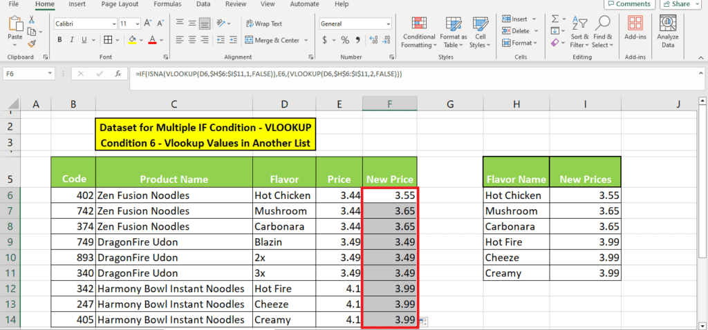
Condition 6 – Using VLOOKUP to fetch values from two tables

While we have discussed how you can use VLOOKUP to return a result based on a single cutoff value, here we discuss how we can use VLOOKUP to return a result based on another table.

We have our product list and prices and another table with updated prices. We need to use VLOOKUP to return whether the price has been changed or not.

Here’s the simple formula for this:

=IF(ISNA(VLOOKUP({Cell address of lookup value},{New table array with $},{Column index number},FALSE)),”No”, “Yes”)

=IF(ISNA(VLOOKUP(D6,$H$6:$I$11,1,FALSE)),”{Return if not found in table}”, “{Return if found in table}”)

Upon pressing “Enter”, here’s the result you will get:

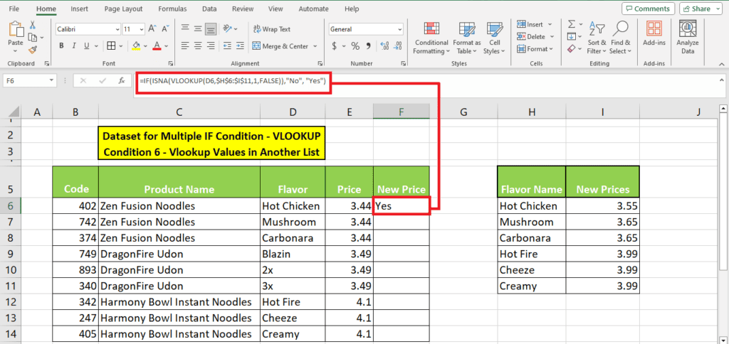
While this formula is simple, it doesn’t help much because it only returns yes and no.

Here’s a modified formula to return the price from the new table or the original price if the product is not found in the new table:

=IF(ISNA(VLOOKUP({Cell address of lookup value},{New table array with $},{Column index number},FALSE)),{Cell Address of old price},(VLOOKUP{Cell address of lookup value},{New table array with $},{Column index number},FALSE)))

=IF(ISNA(VLOOKUP(D6,$H$6:$I$11,1,FALSE)),E6,(VLOOKUP(D6,$H$6:$I$11,2,FALSE)))

By applying another VLOOKUp formula instead of just “Yes”, we can make the formula fetch the new price from the table.

Here’s how this works out:

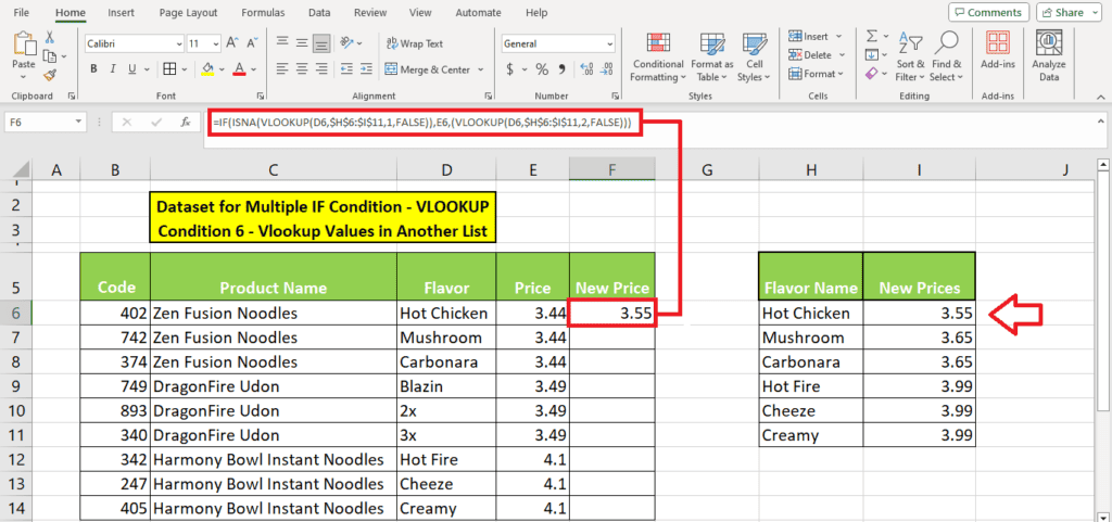
Using the Fill Handle tool, we have the new prices for all flavors present in the updated prices list and old prices for flavors that don’t have updated pricing:

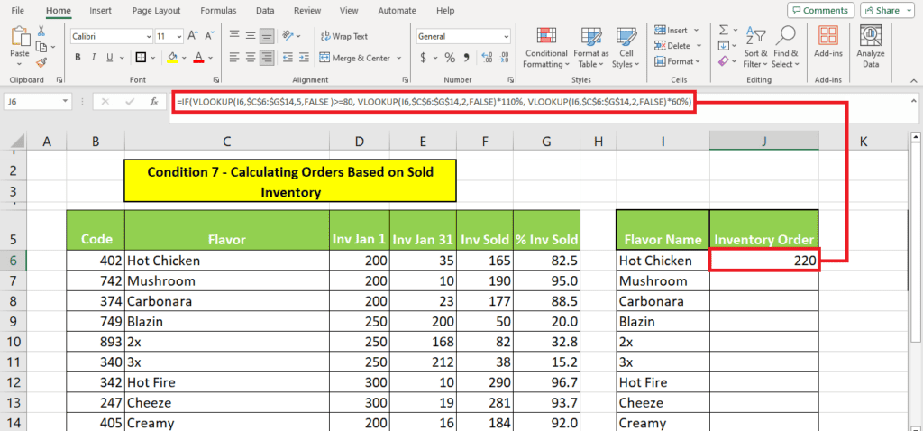
Condition 7 – Using 3 VLOOKUP in 1 IF condition

The superstore wants to order another batch of products. However, it wants to modify the inventory order based on the percentage of inventory sold in January.

They want to increase the inventory order of those products that were sold over 80% by 20%. They want to decrease the inventory order of those products that did not manage to sell 80% of the inventory by 40%.

Instead of manually calculating the amounts, VLOOKUP can help.

But first, some calculations for the inventory sold and the % of inventory sold need to be done in the main table.

After that, VLOOKUP and IF can help calculate the inventory that needs to be ordered.

Here’s the formula syntax for this condition:

=IF(VLOOKUP({Cell address of lookup value},{Table array with $},{Column index number},FALSE)>=percentage, Value if true, Value if false)

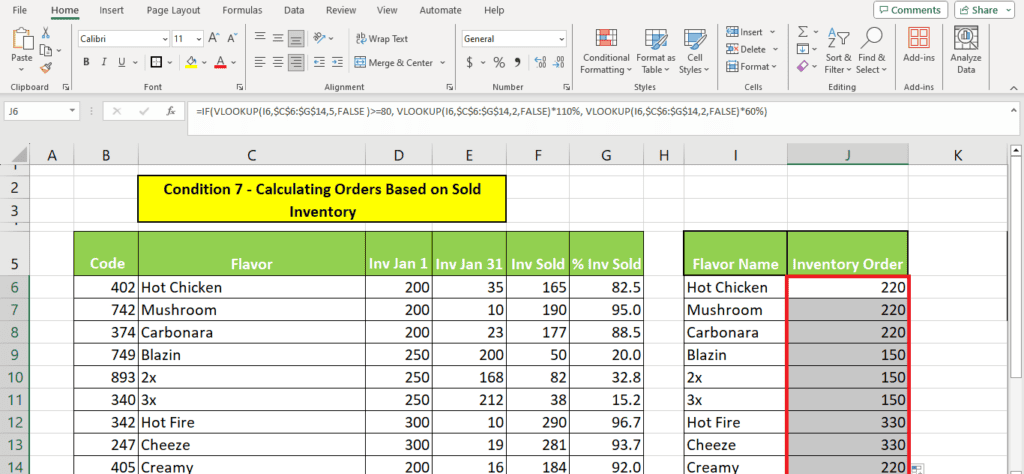
To calculate the “Value if True” and “Value if False”, we need to add two VLOOKUP formulas.

In Value if True, we look up the inventory value in the table and multiply it by 120% to return a 20% increased value.

In Value if False, we look up the inventory value in the table and multiply it by 60% to return a 40% decreased value.

By entering the two new VLOOKUP conditions in the formula, here’s the final formula we get:

=IF(VLOOKUP(I6,$C$6:$G$14,5,FALSE )>=80, VLOOKUP(I6,$C$6:$G$14,2,FALSE)*110%, VLOOKUP(I6,$C$6:$G$14,2,FALSE)*60%)

Here’s the formula in action:

Here’s the result with the formula applied across the inventory table:

Wrapping up

VLOOKUP with the IF formula offers a number of possibilities. We have explored 7 possibilities or conditions in this article, including using VLOOKUP to search for a specific number, using two VLOOKUP formulas in one IF condition, and using three VLOOKUP formulas in one IF condition.

Learn more about the VLOOKUP function through these guides: