How to use VLOOKUP to pull the last match in Excel – 3 ways

If you want to know how to use VLOOKUP to pull the last match in Excel, we’ve got your back.

VLOOKUP’s syntax only returns the first occurrence of the lookup value. However, if you have data where the lookup values have multiple occurrences, the simple VLOOKUP function will not work. To help you out, we have consolidated 4 ways that you can use to use VLOOKUP to return the last occurrence of your lookup value in Excel.

So, without wasting another second, let’s get started!

Using VLOOKUP to fetch the last match in Excel

Scenario on hand: We have a fictional dataset of incoming inventory with dates, product names, and quantity. 

What we want to accomplish: Explore the ways to use VLOOKUP to fetch the last occurrence of the lookup value:

1. Using the LOOKUP function
2. Using the INDEX and MATCH Function 
3. Using the Last Entry Date

Method 1: Using the LOOKUP function

We want to fetch the last inventory update from the dataset. For this, we can use the LOOKUP function.

Here’s the syntax we will use:

=LOOKUP(2,1/({Column array of lookup value}={Cell address of lookup value}),{Column array of return value})

We use the product column instead of the column array of lookup values. 

We use the inventory column instead of the column array of return values. 

Here’s the formula that it makes:

=LOOKUP(2,1/(C6:C13=G6),D6:D13)

Here’s what we get when we input this formula into our sheet:

Using this formula, we can get the last value (300) instead of the first occurrence (550). 

Method 2: Using INDEX and MATCH function 

The INDEX and MATCH functions are often used in place of VLOOKUP for complex situations. We can use this combination in our case as well. 

Here’s the syntax of the INDEX and MATCH functions which we will use:

=INDEX({Column array of return value},MATCH(2,1/({Column array of lookup value column}={Cell address of lookup value}),1))

For our data, we change this syntax to:

=INDEX(D6:D13,MATCH(2,1/(C6:C13=G6),1))

This formula yields the result:

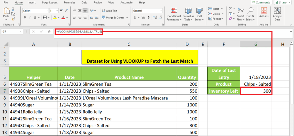
Method 3: Using the last entry date

The last method that you can use to fetch the last entry in the dataset is using the date. 

Using the MAX function, you will first have to fetch the last entry date. 

In our case, it is 1/18/23, as demonstrated below:

To search for both the date and the product name, we need to add a helper column to the left. We simply concatenate the two columns using the following:

={Cell address 1}&{Cell address 2}

Here’s how we apply it to our data:

=B6&C6

Then, using the Fill Handle tool, we will expand this formula across the table:

Then, using this VLOOKUP syntax, we look for the last entry of the product “Chips – salted”:

=VLOOKUP({Lookup value 1}&{Lookup value 2},{Table array},{Column index number},TRUE)

We use TRUE in this formula because the “Chips – Salted” product was not necessarily updated on the latest date. 

Here’s the formula we used for our data:

=VLOOKUP(G5&G6,A6:D13,4,TRUE)

Here’s what we get after entering the formula:

Wrapping up

VLOOKUP pulls the first occurrence of a lookup value. However, this tutorial explores how you use VLOOKUP and other methods to pull the last match in Excel. All of these methods are quite easy. 

Learn more about the VLOOKUP function in Excel through these easy-to-follow guides:

• Excel: How to use column index number in VLOOKUP
• How to perform VLOOKUP between two sheets in Excel
• Finding the second match with VLOOKUP in Excel