Finding the second match with VLOOKUP in Excel – 2 ways


Table of Contents
If you want to learn about finding the second match with VLOOKUP in Excel, you’ve come to the right place.
Manually searching for specific cell values within a range in Excel datasheets can be a cumbersome process. The process can be challenging, especially for beginners. However, this article demonstrates easy methods to identify the second match using the Excel VLOOKUP function.
So, without any further ado, let’s dive in!
How to find second match with VLOOKUP in Excel
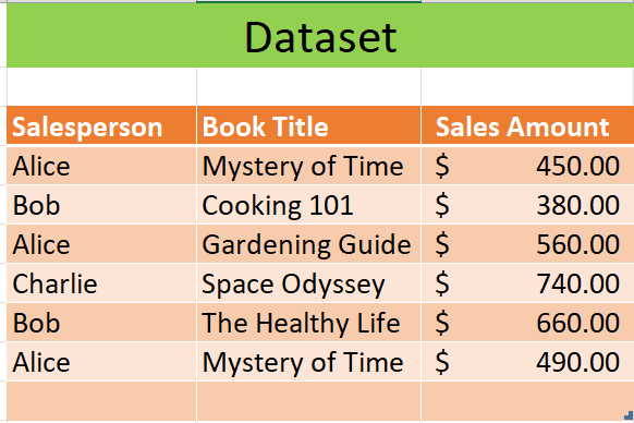
This dataset can be used to demonstrate how to find the second sale made by a particular salesperson for a specific book using VLOOKUP in Excel. The challenge usually is that VLOOKUP by default finds the first match in the dataset.
Parameters:
- lookup_value: The value sought in the leftmost column of the specified table.
- table_array: The table where the lookup_value is searched in its leftmost column.
- col_index_num: The column number in the table from which a value is to be retrieved.
- [range_lookup]: Specifies whether an exact or partial match of the lookup_value is needed. Use 0 for an exact match, and 1 for a partial match. The default is 1 (partial match), and this parameter is optional.
=VLOOKUP(lookup_value, table_array, col_index_num, [range_lookup])
Below are the two ways to look for a second match with VLOOKUP
Method 1 – Finding second match with Excel VLOOKUP & IFNA functions
To find the second sales amount for Alice in our dataset, we would use a combination of the VLOOKUP and IFNA functions along with a helper column to differentiate between the first and second occurrence. Here’s how you can do it step by step:
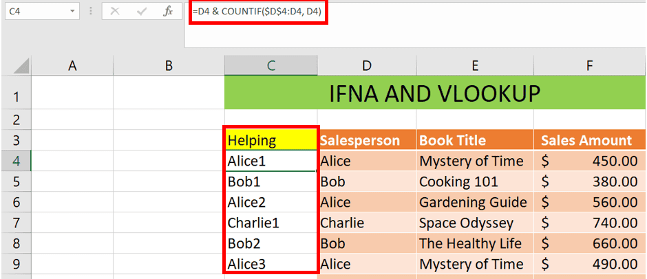
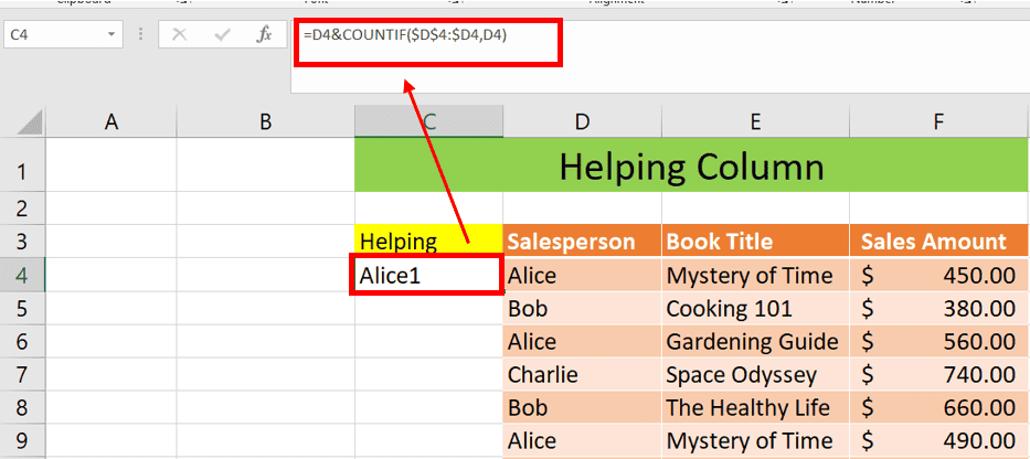
Step 1: Add a Helper Column
- First, you need to create a helper column in your Excel dataset that will keep track of the occurrences of each Salesperson’s name.
- Click on the first cell of the Helper column (let’s say it’s C4, right next to the first salesperson’s name).
- Enter the following formula into cell C4:
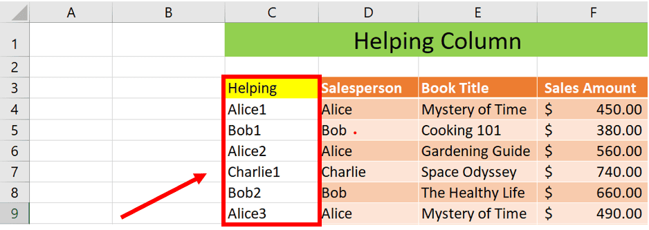
=D4 & COUNTIF($D$4:D4, D4) - Now, press enter and use the AutoFill feature to fill the series.
Step 2: Use VLOOKUP with the Helper Column
- You would use the VLOOKUP function to search for the third occurrence of “Alice” by creating a new search term that includes the number 3 (since you are looking for the third occurrence).
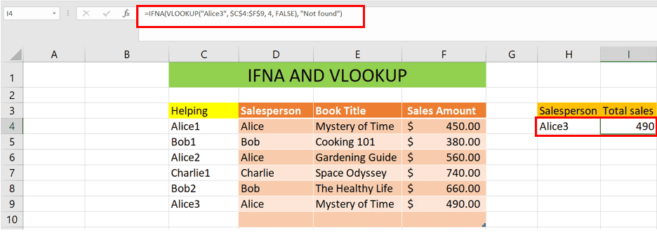
Step 3: Handle Non-Matches with IFNA
- Then, In the formula bar after selecting the cell I4 OR select the cell I4 and type the formula:
=IFNA(VLOOKUP(“Alice3”, $C$4:$F$9, 4, FALSE), “Not found”) - Press enter to get the desired total sales amount for ‘Alice3.
How the formula works
- VLOOKUP(“Alice3”, $B$4:$F$9, 4, FALSE)
This part of the formula searches for the value “Alice3” within the first column of the range $B$4:$F$9. If it finds a match, it returns the value from the 4th column of the matched row within that range.
- IFNA(VLOOKUP(“Alice3”, $B$4:$F$9, 4, FALSE), “Not found”)
This part of the formula essentially does the same as the VLOOKUP part above but includes an error-handling mechanism. The IFNA function captures cases where the VLOOKUP function does not find the “Alice3” value and would normally return a #N/A error. Instead of displaying #N/A, IFNA overrides this with the text “Not found”, thus providing a clear and user-friendly response indicating that “Alice3” does not have a corresponding Sales Amount in the dataset.
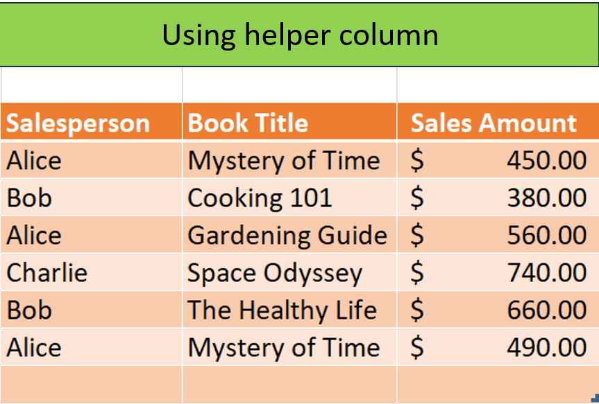
Method 2 – Utilizing a Helper Column to discover the second match with VLOOKUP in Excel
In our initial approach, we’ll set up a Helper Column to easily locate the Second Match using VLOOKUP in Excel.
Let's look at our dataset and look for the total sales for salesperson ‘Bob2.'
Let’s see it step-by-step:
- Select cell C4, or beside the first entry in the salesperson entry, and enter the following formula:
=D4&COUNTIF($D$4:$D4,D4) - You will get an output like this:
- Here, the formula combines B5 with the COUNTIF result in the helper column, creating a unique lookup value. The COUNTIF function tallies Salesman occurrences. Hit Enter, then employ AutoFill to extend the series as illustrated below.
- After selecting the cell I4 or the cell you want the corresponding value, paste the following formula replacing it with your desired cell and cell ranges.
=VLOOKUP(“Bob”&2,C3:F10,4)
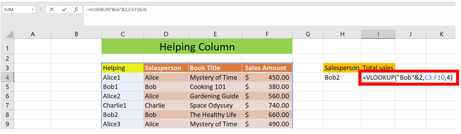
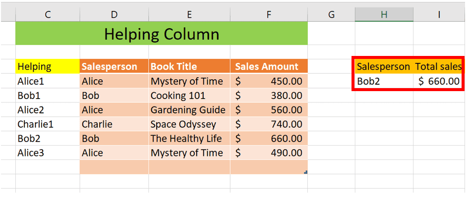
- In this VLOOKUP formula, it looks for a match for Bob2 and returns back the sales amount from the column. You can press enter and see the results.
Conclusion
In conclusion, these two straightforward methods offer a simple way to find the second match using VLOOKUP in Excel. Whether utilizing a helper column or an array formula, these approaches enhance efficiency in locating specific data points within your Excel datasets.
Learn more about the VLOOKUP function in Excel with these in-depth guides:
- Guide to VLOOKUP Fuzzy Match in Excel
- How to return the highest value using the VLOOKUP function in Excel
- How to use VLOOKUP to search text in Excel
About the Author