
How to freeze rows and columns in Excel – our step-by-step guide

Reviewed By: Kevin Pocock

Table of Contents
If you want to learn how to freeze rows and columns in Excel, then you’ve landed on the right page.
Freezing rows or columns in Excel can be a great idea when you have a lot of information on a spreadsheet and need to remember certain data while you continue working. Freezing a row or column will allow it to stay on the screen no matter how far you scroll, and it is a great built-in feature that will prevent you from writing down equations or statistics vital to the end result.
Prime Day is finally here! Find all the biggest tech and PC deals below.
- Sapphire 11348-03-20G Pulse AMD Radeon™ RX 9070 XT Was $779 Now $739
- AMD Ryzen 7 7800X3D 8-Core, 16-Thread Desktop Processor Was $449 Now $341
- ASUS RTX™ 5060 OC Edition Graphics Card Was $379 Now $339
- LG 77-Inch Class OLED evo AI 4K C5 Series Smart TV Was $3,696 Now $2,796
- Intel® Core™ i7-14700K New Gaming Desktop Was $320.99 Now $274
- Lexar 2TB NM1090 w/HeatSink SSD PCIe Gen5x4 NVMe M.2 Was $281.97 Now $214.98
- Apple Watch Series 10 GPS + Cellular 42mm case Smartwatch Was $499.99 Now $379.99
- ASUS ROG Strix G16 (2025) 16" FHD, RTX 5060 gaming laptop Was $1,499.99 Now $1,274.99
- Apple iPad mini (A17 Pro): Apple Intelligence Was $499.99 Now $379.99
*Prices and savings subject to change. Click through to get the current prices.
As the option to freeze rows and columns is hidden behind a layer of settings, we’ll walk you through the entire process to make things easier for you.
Here’s how to freeze a row or column in Excel
If you want to freeze rows or columns, follow these steps.
Step
Highlight a row or column
When you open up the Excel document you want to start editing, click on the row or column you want to freeze.
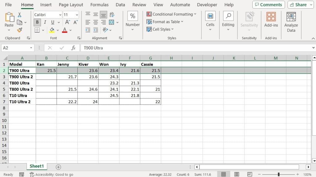
The way this works is if you highlight a row or column, all others rows above or columns on the side will be frozen. For example, if you choose row 5, the 4 previous rows will also be frozen on your screen, allowing you to get a bulk of information saved at once.
Step
Click on the View tab
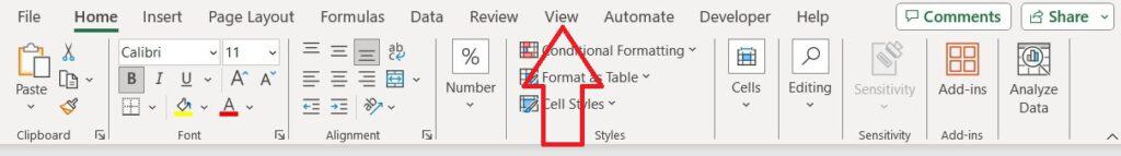
When you have chosen the rows or columns you want to freeze, there will be a handful of options at the top that you can click on.
Each has their own set of tools that can be used to format a sheet in different ways and can really open up all the potential features an Excel user has at their disposal.
The option you will want to click on is ‘View' near the far right of the screen.
Step
Select Freeze Panes
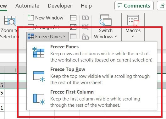
Once the ‘View' menu has been selected, look to the far right at the top of the screen to see a ‘Freeze panes' option. Click on the small arrow beside it to open a drop-down menu.
Step
Choose to freeze rows/columns
You will be offered three options, two of which are to only freeze the top row or first column.
Instead, click the first option simply called ‘Freeze Panes' to tell Excel to freeze only the rows that had been selected previously.
Step
How unfreeze works
Your rows of choice will now be frozen and be easy to see as you navigate the page.
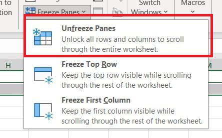
If you ever feel the rows are a bit too cumbersome or you don't need them anymore, simply go on the same ‘Freeze Panes' drop-down menu and click ‘Unfreeze Panes'.
Conclusion
Freezing multiple rows at a time is a quick and easy way to keep a few crucial bits of information memorized and ready to go whenever you may need them throughout your work. Excel makes this function extremely easy to toggle on and off, which is part of the reason it has become the most popular spreadsheet platform.
If you want to learn more about Excel and how it works, give these guides a read:
- How to remove gridlines in Excel
- How to sum cells with text and numbers in Excel
- How to insert rows in Excel
About the Author