How to sum cells with text and numbers in Excel – 3 methods

If you want to know how to sum cells with text and numbers in Excel, we’ve got you covered.

Dealing with numbers in Excel is usually a breeze, but things can get tricky when these numbers are tucked in with text, like dollar signs with prices or pieces with quantities. If you’re scratching your head over how to add these mixed cells, don’t worry; it’s not as tough as it seems.

In this guide, we will discuss how to sum cells with text and numbers in Excel using three different methods.

Method 1: Using LEFT and FIND functions to sum cells with text and numbers

When working with Excel, combining text and numbers within the same cell is common. For example, in our inventory list, we have quantities of items with the word “units” appended to the number. To sum up these mixed cells, we must first isolate the numerical part. This is where Excel’s text functions, like FIND and LEFT, come into play, along with the VALUE function to convert text to numbers and the SUM function to add them all up.

Let’s have a look at our dataset:

FIND function

The FIND function in Excel is used to locate the position of a specified text within another text string. The syntax for the FIND function is:

=FIND(find_text, within_text, [start_num])

• find_text: The text you want to find.
• within_text: The text string you want to search within.
• start_num [Optional]: The character position in the within_text string from which to start the search. The default value is 1, indicating the function should start searching from the first character.

In our scenario, we use the FIND function to locate the position of the word “units” within the text string in each cell of the “Quantity in Stock” column (D4:D8). This helps us determine where the numeric part of the string ends.

LEFT function

The LEFT function extracts a specified number of characters from the left side of a text string. Its syntax is:

=LEFT(text, [num_chars])

• text: The text string from which you want to extract characters.
• num_chars [Optional]: The number of characters to extract, starting from the leftmost character. If omitted, the default is 1.

In our case, we combine the LEFT function with the FIND function to extract just the numeric part of our “Quantity in Stock” data by taking characters from the left up to the position just before where the word “units” is found.

VALUE function

The VALUE function is used to convert a text string that represents a number into a numerical value. Here’s the syntax:

=VALUE(text)

• text: The text string that you want to convert into a number.

In our dataset, we use the VALUE function to convert the numeric text extracted with the LEFT function into a number that Excel can recognize and calculate.

Combining the functions

In the provided dataset, you want to sum the quantities in the “Quantity in Stock” column, which is in the format of “number units.” To do this, we first isolate the numeric part using LEFT and FIND, then convert these numeric strings to actual numbers with VALUE, and finally, add them up with SUM:

=SUM(VALUE(LEFT(D4:D8, FIND(” units”, D4:D8)-1)))

Here’s a step-by-step breakdown of our dataset:

1. FIND(” units,” D4:D8) finds the starting position of the text ” units” within each cell from D4 to D8.
2. LEFT(D4:D8, FIND(” units,” D4:D8)-1) extracts the number from each cell, which is positioned to the left of the text ” units.”
3. VALUE(LEFT(…)) converts the extracted numeric text to actual numeric values.
4. SUM(VALUE(…)) adds up all the numeric values to give us the total quantity in stock.

This formula should be entered into the cell where you want the total sum to appear, in this case, D9. If you’re not using an Excel version that automatically processes array formulas (such as Excel 365 or Excel 2021), remember to confirm this formula as an array formula by pressing Ctrl + Shift + Enter.

After pressing Enter, we will get the sum of our Total Stock, which is 195 in our case.

Method 2: Summing cells containing text and numbers with the SUBSTITUTE function

First, let’s take a look at our dataset to see how we can use the SUBSTITUTE function to calculate the total stock:

SUBSTITUTE function overview

The SUBSTITUTE function in Excel replaces existing text with new text in a string. The syntax for the SUBSTITUTE function is:

=SUBSTITUTE(text, old_text, new_text, [instance_num])

• text: The string or cell reference containing the text you want to change.
• old_text: The sequence of characters you want to replace.
• new_text: The sequence of characters that will replace old_text.
• instance_num [Optional]: Specifies which occurrence of old_text you want to replace with new_text. If omitted, every instance of old_text is replaced.

Using the SUBSTITUTE function to prepare for summation

When you have cells that combine numbers and text (such as “10 units”), you can use SUBSTITUTE to remove the text part, leaving only the numbers, which can then be summed.

Applying SUBSTITUTE in our dataset

1. Identify the text to remove: In your dataset, we want to remove the word “units” from the “Quantity in Stock” column to isolate the numerical values.
2. Use SUBSTITUTE to replace text with an empty string: We’ll use SUBSTITUTE to replace “units” with an empty string (“”).
   =SUBSTITUTE(D4:D8, ” units”, “”)
3. Convert the resulting text to numbers: After removing the text, we still have numbers in text format. To sum them up, we need to convert them to numerical values using the VALUE function.
   =VALUE(SUBSTITUTE(D4:D8, ” units”, “”))
4. Sum the converted numbers: Lastly, we sum up these values with the SUM function.
   =SUM(VALUE(SUBSTITUTE(D4:D8, ” units”, “”)))
5. Click on the cell where you want the total to appear, cell D9 in your case.
6. Enter the above formula
7. Press Enter to get the total sum OR (  Ctrl + Shift + Enter ).

Note: If you’re using an Excel version that doesn’t automatically handle array formulas, you need to enter the formula as an array formula. You do this by pressing Ctrl + Shift + Enter instead of just Enter. This will surround your formula with curly braces {} to indicate it’s an array formula.

And there you have it! This formula will calculate the total stock by summing the numbers in the “Quantity in Stock” column after removing the text ” units” from each cell.

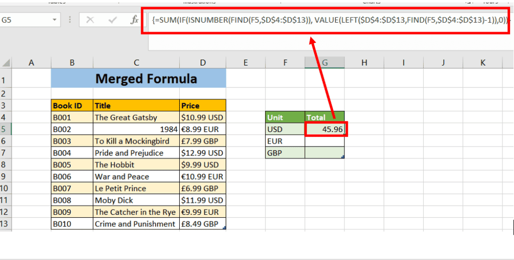
Method 3: Using a merged formula strategy

To calculate the total Amount (GBP, US, EURO )  in Excel, we can use a combination of Excel functions: SUM, IF, ISNUMBER, SEARCH (or FIND), and LEFT. Here’s how to create a formula for each unit based on the dataset structure you’ve described:

• SUM Function: Adds up all the numbers in a range or array.
• IF Function: Checks a condition and returns one value if the condition is true and another value if the condition is false.
• ISNUMBER Function: Determines if a value is a number, returning TRUE or FALSE.
• SEARCH (or FIND) Function: Finds one text string within another, returning the position of the first occurrence. SEARCH is not case-sensitive, whereas FIND is.
• LEFT Function: Extracts a given number of characters from the left side of a text string.

Let’s consider our dataset:

Our dataset consists of a list of books with their prices in multiple currencies. The “Price” column combines numerical values with currency labels.

Select Cell G5 and insert the following formula:

=SUM(IF(ISNUMBER(FIND(F5,$D$4:$D$13)), VALUE(LEFT($D$4:$D$13,FIND(F5,$D$4:$D$13)-1)),0)

Now let’s see what our formula means:

• FIND(F5, $D$4:$D$13): This part of the formula searches for the text in cell F5 (which is “USD”) within the range D4:D13, which contains the prices of books with their currency codes.
• ISNUMBER(…): This function is used to check if the result of the FIND function is a number. Since FIND returns the position at which the searched string starts, if it finds the string, it will return a number (position), and ISNUMBER will return TRUE. If the string is not found, FIND will return an error, and ISNUMBER will return FALSE.
• LEFT($D$4:$D$13, FIND(F5, $D$4:$D$13) – 1): This part of the formula extracts the substring from the left side of each price in the range D4:D13 up to (but not including) the position where the currency code starts (determined by the FIND function). This effectively gives you the numeric part of the price without the currency code.
• VALUE(…): This function converts the text returned by the LEFT function into a number so it can be used in mathematical operations.
• IF(ISNUMBER(FIND(F5, $D$4:$D$13)), VALUE(LEFT($D$4:$D$13, FIND(F5, $D$4:$D$13) – 1)), 0): This IF statement checks each cell in the range D4:D13. If the currency code in F5 is found within the cell, it converts the price to a number; otherwise, it returns 0.
• SUM(…): Finally, this function adds up all the numbers generated by the IF function.

In summary, the formula is checking each price in the range D4:D13 to see if it includes the currency code “USD” from F5. If it does, it strips out the currency code, converts the remaining text to a number, and adds it to the sum. If the currency code is not found, it adds 0 for that cell. The result is the sum of all prices in USD from the list in D4:D13.

Sum cells using text

When working with Excel, summing cells that contain text is a common task that can be performed using various functions. The COUNTIF function is particularly useful for counting the number of occurrences of specific text within a range of cells. Below, we demonstrate how to use the COUNTIF function to sum cells with text.

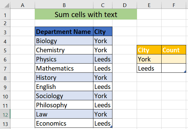
We want to calculate the sum (count) of departments located in each city and display the result in Column F with the column header as ‘Count.’

Process to SUM cells with text in Excel

• First, enter the following formula in cell F6:

=COUNTIF($C$4:$C$13,E6)

Here, C4:C13 refers to the cells under the ‘City’ column, and E6 is the city for which we want to count the departments, for example, ‘York.’

• After writing the formula, press ENTER to get the count for the first city.

By following these steps, you will get the count of departments for each city listed in your dataset. This method is efficient and easily adaptable to various data ranges.

Conclusion

This was how to sum cells with text and numbers in Excel. To wrap it up, adding numbers in Excel that are mixed with words is easy once you know how. With simple tricks like LEFT, FIND, or SUBSTITUTE, you can pull out the numbers you need and add them up quickly.

Learn more about Excel through these helpful guides:

• How to remove gridlines in Excel
• How to check your Excel version
• How to insert rows in Excel