Table of Contents
When you are using Excel you may find that you have a large spreadsheet that requires some scrolling to get a good look at all the data. When comparing data in this way you may want to still see the row headings, or even a column, while you move around a large spreadsheet.
Freezing panes in Excel allows you to keep certain areas of the worksheet visible while you scroll around the worksheet. This can work with both horizontal and vertical scrolling and is a really useful way to save time and compare data efficiently.
How To Freeze Panes
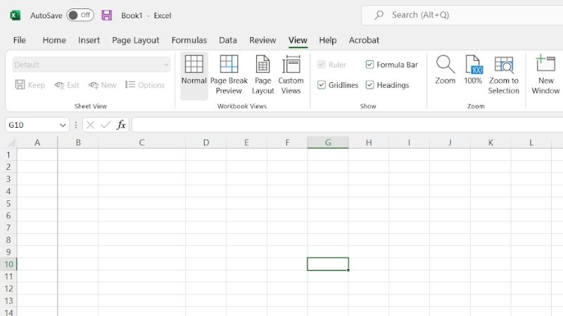
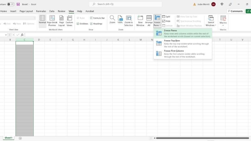
In the ‘View' tab there is a ‘Window' area. Within this area there are a few options, the only one you need to freeze panes is the ‘Freeze Panes'. There are a few options here that isolate different bits of the table we will explain below.
Step
Freezing The First Column Of A Spreadsheet
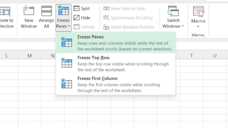
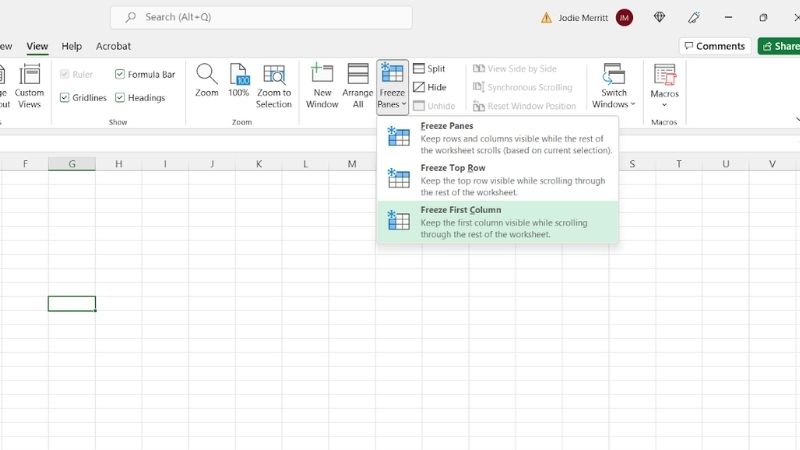
Simply select the ‘View' and click the ‘Freeze Panes' drop down menu.
There are a few options in the drop-down menu, to freeze the first column select ‘Freeze First Column'.
Try scrolling across, you should see that this column won't disappear no matter where you are on the sheet.
A visible line separating column A and B should show that the column has been frozen.
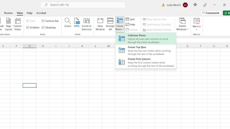
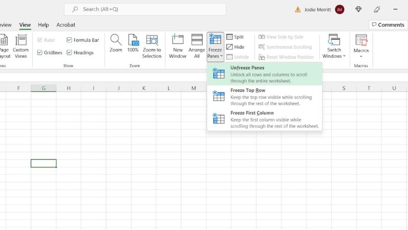
To unfreeze simply follow the same steps and select the ‘Unfreeze Panes' button.
Step
How To Freeze The First Two Columns
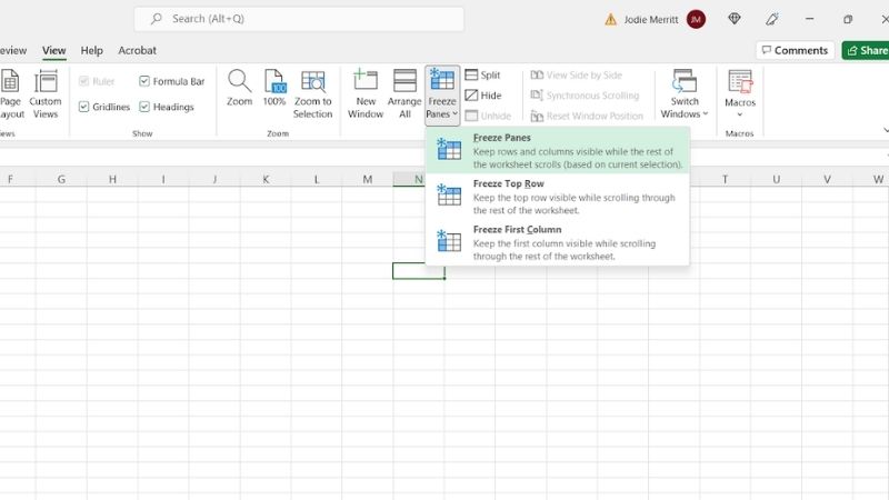
To freeze the first two columns you, counter intuitively, need to select the third column. In practice always remember the ‘Freeze' function will freeze what is behind the column you have selected.
Select the ‘View' tab and then the ‘Freeze Panes' drop down menu, then select ‘Freeze Panes' within that.
This can work for any number of cells, just follow the simple rule of clicking the column in front of what you are wanting to freeze. For example if you want to freeze the first 5 columns, select the sixth.
Step
How To Freeze Columns And Rows
This is a super helpful way to keep your data comparisons accurate, it allows you to see both the headers of each column as well as the first column. This step can apply to any number of columns or rows you want to freeze.
To freeze rows and columns select the cell which is below the rows you want to freeze and to the right of the columns you want to freeze. This means whatever is above and also behind the cell selected will be frozen.
Select the ‘View' tab and then select the ‘Freeze Panes' drop down menu, then select the ‘Freeze Panes' option. Go back into this drop down menu and select ‘Unfreeze Panes' when you want to unfreeze the panes.
In Summary
If you cannot find the ‘View' tab you may be using a free version of Excel called Excel starter. You must purchase the full version of Excel in order to use the ‘Freeze Panes' function.
The freeze pane function on Excel is really helpful and is another tool to make your data management and comparisons a lot more efficient and also quick.
Moreover, having the free pane function allows you to also keep your data comparisons accurate. Most data issues on Excel often occur as people try to remember the heading of each cell or the name of a cell while they are scrolling. Relying on your memory isn't the best course of action when analyzing lots of data for a long time.
Hopefully these steps can make you a more efficient user of Excel.
About the Author
