How to compare two columns in Excel – 6 simple methods

Last Updated on March 6, 2024

If you want to know how to compare two columns in Excel, you’ve landed on the right page.

Excel is a spreadsheet software program that you can use to deal with massive databases. But it doesn’t only serve as a program to store data, as you can use different formulas to make calculations and even compare data. However, the process can seem tricky for some people, especially if they are new to Excel.

This is where we come in. In this guide, we will go over six different methods that can help you compare two columns in Excel. So, without wasting another second, let’s dive in!

How you can compare two columns in Excel

Scenario on hand: We have a supermarket dataset in Excel.  

What we want to accomplish: Explore how to compare two columns in Excel using the following ways:

1. Exact match using the IF formula
2. Case-sensitive differences in columns
3. Compare two lists in Excel 
4. Compare two lists using INDEX and MATCH
5. Compare two lists with ‘Find & Select’
6. Compare two lists for partial matches

Exact match using the IF formula

You can easily compare two columns in Excel using the IF() formula. This formula compares two values and returns either TRUE or FALSE, depending on whether they match.

For this method, simply type the formula:

IF(cell address 1=cell address two,{“Value if true”},{“Value if false”})

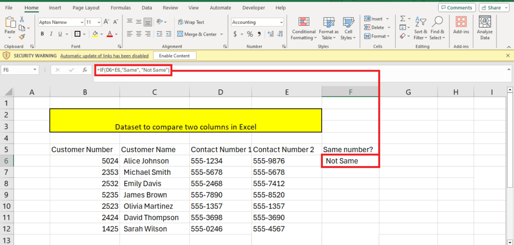
Our dataset has customer names with two contact numbers for each customer. However, some customers have given one contact number twice. To check this, we use this formula:

=IF(D6=E6,”Same”, “Not Same”)

Here’s the result we get for the first cell:

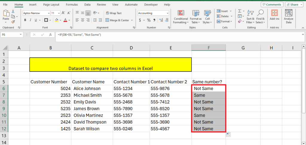
We drag this formula to the rest of the table using the Fill Handle Tool, a small square at the bottom left of the cell. To use it, we press down the cursor and drag it to the rest of the table before releasing it. Excel dynamically changes the formula to compare each row in a similar fashion:

Case-sensitive differences in columns

When handling data, you should ensure that your data is in the same format. However, in data entry, people may enter in all caps or keep the first letter capitalized. This trick can come in handy to ensure that your data is uniform. 

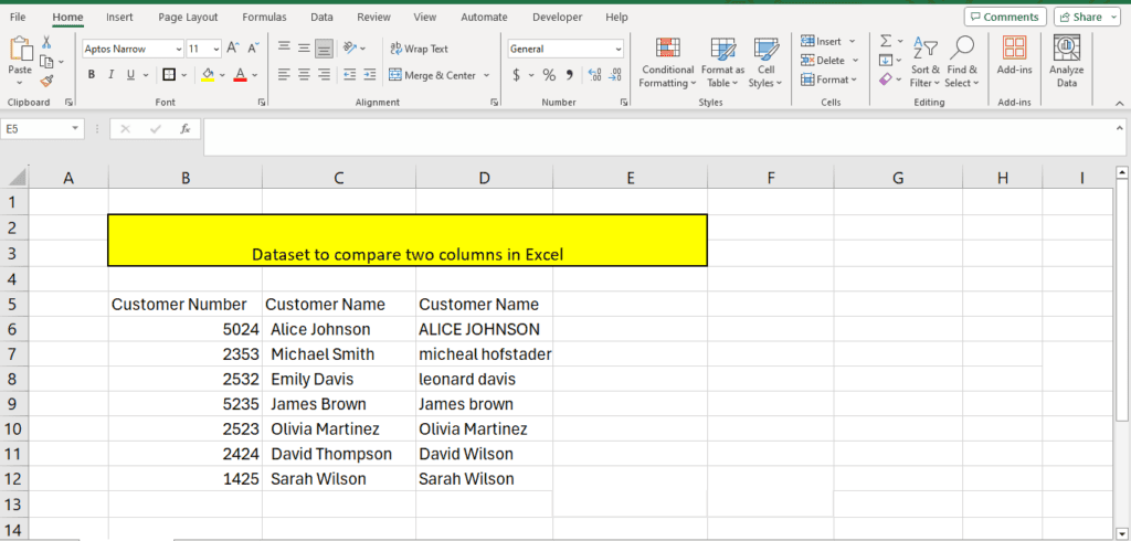
Let’s consider two columns with data. Some of these columns have matching data, while others are matching but have case differences.

To see if the names are a case-sensitive match, we use the IF(EXACT combination. Here’s the syntax for this formula:

=IF(EXACT(cell address 1, cell address 2), “{Value if matching}”, “{Value if not matching}”)

For our dataset, we use the formula like this:

=IF(EXACT(C6, D6), “Match”, “Unique”)

Here’s the result:

Compare two lists in Excel 

The two methods above are for comparing the columns row-by-row. However, there will be very few cases when you find data matching row-by-row. 

Most times, you will have two separate lists and will have to find the duplicate values amongst them. The IF and IF(EXACT) formula wouldn’t work in this case. 

Here’s a simple way to compare two tables or columns using VLOOKUP. 

Simply write the following IF(VLOOKUP formula:

=IF(VLOOKUP({cell address of lookup value},{column array with absolute references},1,FALSE)={cell address of lookup value},”Duplicate”)

=IF(VLOOKUP(D6,$C$6:$C$12,1,FALSE)=D6,”Duplicate”)

Here’s what we get for a table with two customer columns:

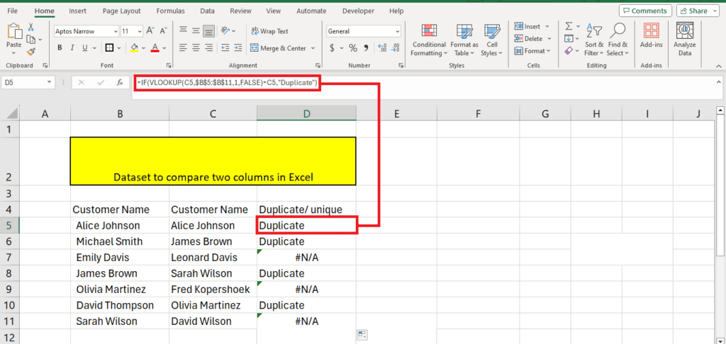
This formula takes one value and looks through it in the other list. If it is repeated in the list, the formula returns “Duplicate.” If it doesn’t find a match, it gives an #N/A error. 

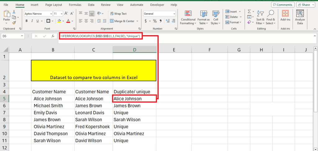
If you wish to remove the #N/A error, use IFERROR instead of IF. Here’s how the modified formula looks like:

=IFERROR(VLOOKUP(C5,$B$5:$B$11,1,FALSE),”Unique”)

This returns the name of the person if it finds a duplicate match and “Unique” if it does not find a match:

Compare two lists using INDEX and MATCH

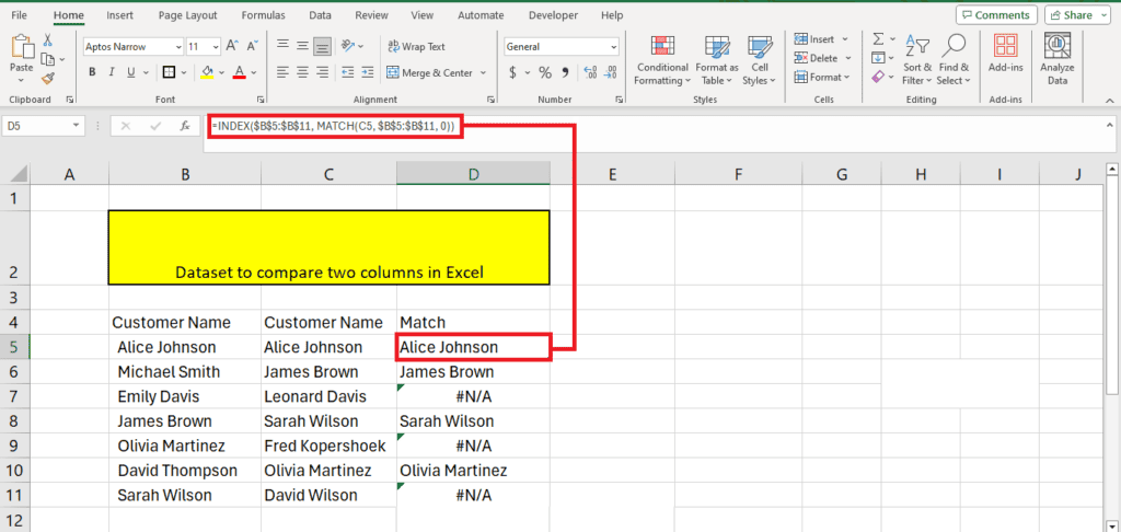
You can use the VLOOKUP formula to return duplicate values in a third column. You can also do the same using an INDEX and MATCH formula. 

This method is also quite simple. Here’s the syntax it uses:

=INDEX({column array with absolute references}, MATCH({Cell address to lookup}, {column array with absolute references}, 0))

Here’s what the formula we used for our dataset:

=INDEX($B$5:$B$11, MATCH(C5, $B$5:$B$11, 0))

Here’s the result we get:

Compare two lists with ‘Conditional Formatting’

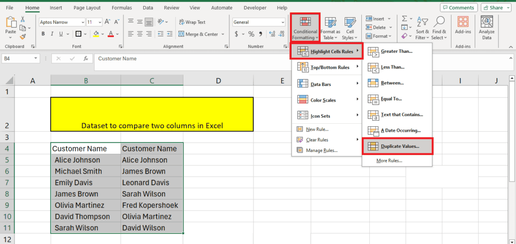
Another great way to identify unique and duplicate values in your rows is by using the ‘Conditional Formatting’ option found in the Home tab. 

To use this option, first select both the columns you want to compare. Then, click ‘Conditional Formatting’ > Highlight cell rules > Duplicate Values:

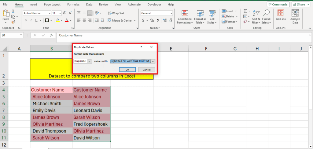
This will open up a window where you can select the highlight color for duplicate values:

Compare two lists for partial matches

You can even compare two lists for partial matches. We changed the dataset a bit for this demonstration to include the customers’ numbers. 

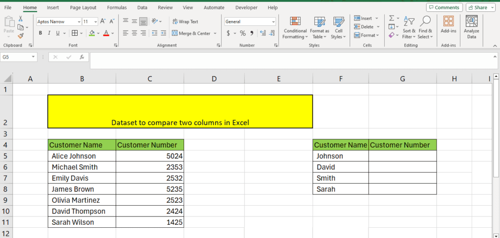
We need to look up the partial values from column F and fetch the values they correspond with from the original table. 

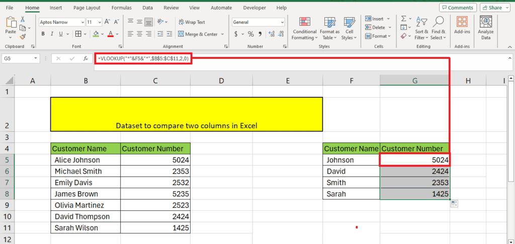
Here’s the VLOOKUP formula we use for this:

=VLOOKUP(“*”&F5&”*”,$B$5:$C$11,2,0)

In this formula, we use the wildcards “*”& on either side of the cell address of the lookup value to get a partial match from the dataset. Here’s the result we get using this formula:

Wrapping up

There will be many times when you have to compare two columns in Excel. You can use formulas to find exact matches in columns. You can also use an IF and EXACT formula to find case-sensitive matches. While there are different ways to compare columns in Excel, as long as you have the appropriate formulas, you can get your work done.

If you want to learn more about Excel, give these guides a read:

• How to edit a drop-down list in Excel
• How to print address labels from Excel
• How to lock a column in Excel