Last Updated on
SUMIF is one of the most crucial functions in the Microsoft Excel tool belt. You’ll use it to automatically add together data entries based on the criteria of your SUMIF command, saving you from combing through endless reams of info and adding all relevant figures manually.
The SUMIF process can look a little intimidating at first, but we’re here to show you that it’s a piece of cake.
Read on to take your Excel skills to the next level (and then some!).

SUMIF Syntax
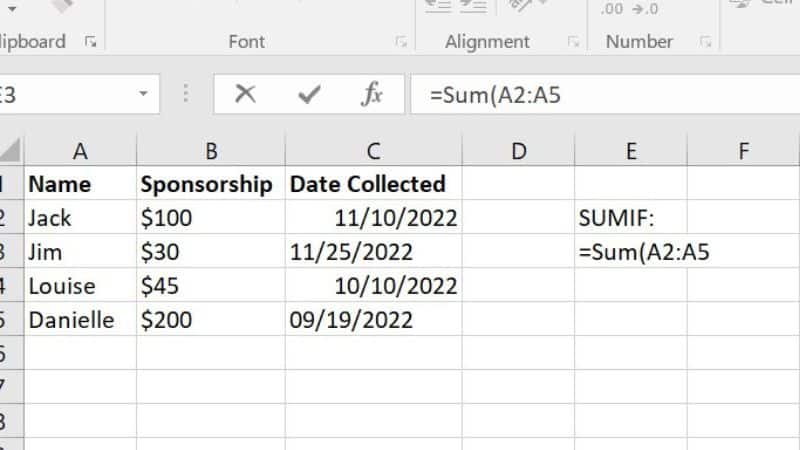
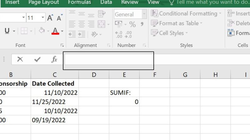
You can type your formula into an empty cell of your choice and you will see it appear in the formula bar, which is highlighted below.

But before you go in guns blazing, you need to know the syntax, or order, of the SUMIF formula, which is as follows:
=SUMIF
The = symbol tells Excel you’re typing in a function, and SUMIF tells it which one.
Range
This establishes the range of cells you wish to evaluate. The cells must contain at least some numerical data, the formula should begin with open parentheses, and you must separate your coordinates with a colon.
For example, if you wanted SUMIF to evaluate cells A1 to A5, your range would be expressed like so: (A1:A5. Thus far, altogether, you have…
=SUMIF(A1:A5
Criteria
So, Excel now knows where to look, but it doesn’t know what it’s looking for, so you need to tell it.
For instance, let’s say that you’re looking at a list of property values, and you need the sum of all values exceeding $200,000. Your criteria would be expressed “>$200000”, leaving our formula looking a little something like this:
=SUMIF(A1:A5,“>$200000”
However, you’re not limited to cell values when selecting your criteria. It could be cell references, function, or expression. You can also use “wildcard” characters in the criteria, e.g. (?) to match any single character or (*) to match any sequence of characters.
To search for criteria that actually include the wildcard character, precede it with a tilde (̴).
Sum_Range
Sum_range is an optional addition that you may not need to use. It essentially overwrites the established range with a new cell range that corresponds with the first. As these two ranges are correlated, the new range must match the sample size of the first.
For example, if our range is A1:A5, our sum range could be B1:B5, and the SUMIF function would use A1:A9 as the general range of inquiry, but the answer would be given from the sum_range in relation to the range.
With this sum_range, our complete formula would end up looking like this:
=SUMIF(A1:A5,“>$200000”,B1:B5)
Our Example In Action
Let’s say our two Excel columns look like this…
| Property Prices | Commission |
| $100,000 | $10,000 |
| $300,000 | $30,000 |
| $500,000 | $50,000 |
| $600,000 | $60,000 |
| $700,000 | $70,000 |
… and we typed the following formula into our free cell:
=SUMIF(A1:A5“>$200000”)
… then pressed Enter; our total would be $2,100,000.
But if we included our sum_range from earlier:
+SUMIF(A1:A5“>$200000”,B1:B5)
Our total would be $210,000, drawn from the “Commision” column.
Final Thoughts
The “IF” suffix diversifies the SUM function a great deal, making large, complex fields of data easy to work with and analyze, but it can be a bit of a mind-bender at first.
Our advice is to open up Excel, make a very simple worksheet like our example above, and practice with your newfound ability — you’ll have it down in no time!

