
If you want to learn how to sort a bar chart without sorting data in Excel, then you’ve landed on the right page.
In Excel, when handling worksheets filled with sales figures, it often becomes necessary to visualize data in a sorted manner through a bar chart without actually rearranging the underlying data. This approach helps comprehend the sales trends in ascending or descending order without tampering with the original dataset.
Sorting a bar chart while keeping the dataset intact is not only straightforward but also a great way to save time and maintain data integrity. And in this guide, we will explore three efficient and easy steps to achieve this in Excel.
How you can sort a bar chart without sorting data
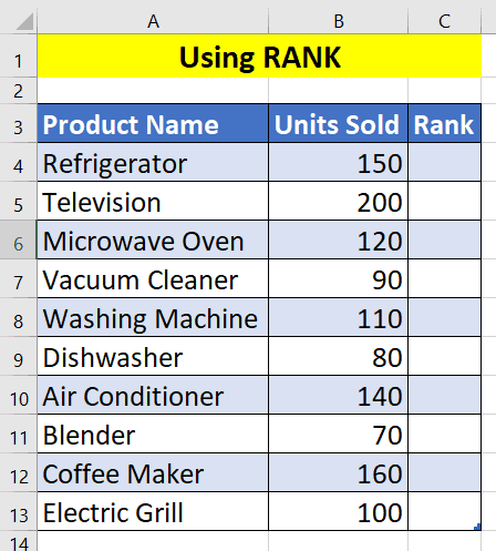
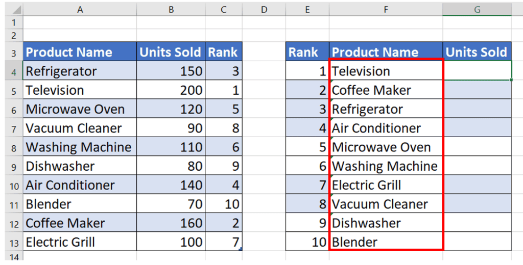
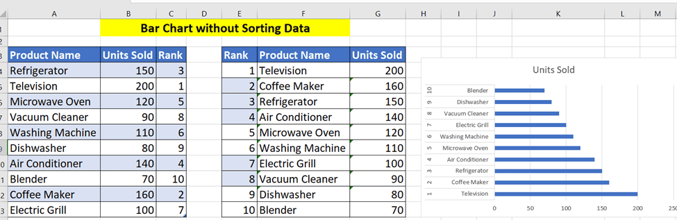
Imagine we have a dataset from the sales department of the XYZ Corporation. This dataset includes a list of products with corresponding units sold that have already been ranked based on their sales performance. The information is laid out neatly across columns A and B, with the rankings specified in column C. Our objective is to construct a bar chart that reflects the sales data in either ascending or descending order without altering the original arrangement of the data. We will utilize Excel’s powerful RANK, INDEX, and MATCH functions to accomplish this. These functions will allow us to visualize the data effectively while preserving the original dataset’s structure.
Step 1: Use a RANK Function
In this step, we’ll use the RANK function in Excel to organize our bar charts while keeping our dataset unchanged. This method is particularly useful when you want to visualize data according to their rank but wish to leave the original data sequence intact. Here’s how we can proceed with the given dataset.
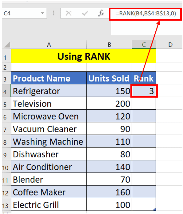
- Firstly, we’ll select cell C4 to start applying the RANK function right next to our ‘Units Sold’ data for the ‘Refrigerator’.
- The formula we’ll use in cell C4 is as follows:
=RANK(B4, $B$4:$B$13, 0)
In this formula, B4 represents the ‘Units Sold’ for the ‘Refrigerator,’ $B$4:$B$13 is the range of the ‘Units Sold’ for all products, and 0 denotes that we are sorting in descending order. The dollar sign ($) is used to create an absolute reference, which ensures that when we copy the formula down the column, the reference to our range remains constant.
- Upon pressing ENTER, cell C4 will display the rank for the ‘Refrigerator’ based on the units sold.
- Next, we’ll use the AutoFill feature to extend the RANK function to the rest of the cells in column C. Simply drag the fill handle from C4 down to C13 to apply the formula to all products.
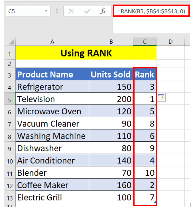
As a result, each product will have a rank assigned according to the number of units sold, allowing us to create a bar chart that is sorted by these ranks without altering the original order of our data. The final outcome will be a neatly organized bar chart, with the products ranked from highest to lowest or vice versa, depending on the chosen sort order. The process ensures that the dataset in columns A and B remains as shown above while our visual representation is sorted.
Step 2: Merge INDEX and MATCH functions for ascending-order sorting
For our given dataset, we’re going to utilize the INDEX and MATCH functions to sort the bar chart data without changing the underlying dataset. This is a powerful technique to visually represent data in an ordered fashion without disrupting the original data layout. Here’s how we can apply these functions to our sales data:
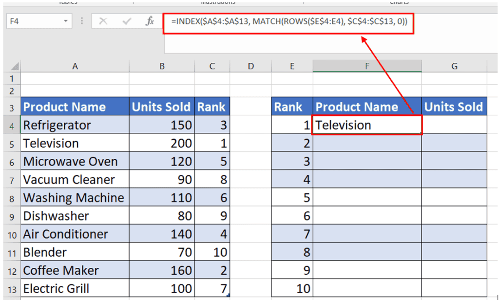
- Initially, we’ll select cell D4. This is where we’ll input our combined INDEX and MATCH formula to determine the corresponding ‘Units Sold’ for each ‘Product Name’ based on its rank.
- Here is the formula we’ll use in cell C4:
=INDEX($A$4:$A$13, MATCH(ROWS($E$4:E4), $C$4:$C$13, 0))
- After pressing ENTER, cell D4 will display the ‘Units Sold’ for the product with the lowest rank.
Formula Breakdown:
- MATCH(ROWS($E$4:E4), $C$4:$C$13, 0) finds the position of the rank number in the range $C$4:$C$13. ROWS($E$4:E4) will increase as we drag the formula down, giving us sequential ranks starting from the smallest rank.
- INDEX($A$4:$A$13, …) then returns the ‘Units Sold’ value from the range $A$4:$A$13 that corresponds to the rank position found by the MATCH function.
- Then, we’ll use the AutoFill feature to copy this formula down from F4 to F13. As a result, column F will display the ‘PRODUCTS’ in ascending order of rank, while the original Units sold data in column B remains unchanged.
- Now, we’ll move to the next step, which involves repeating a similar process to sort the ‘Units Sold’ in accordance with the rank. Select cell G4 and enter the following formula:
=INDEX($B$4:$B$13, MATCH(ROWS($E$4:E4), $C$4:$C$13, 0))
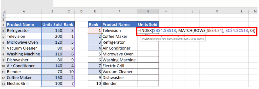
- After entering this formula and using the AutoFill feature again, column G will list the ‘Units Sold’ sorted by the ascending order of their sales rank.
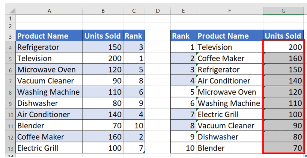
By completing these steps, we’ll have a new range of cells (D4:E13) displaying our sorted bar chart data by rank, without altering the original data sequence in columns A and B.
Step 3: Build an unsorted data bar chart
Now, let’s proceed to visually sort our bar chart using the dataset we’ve prepared without actually rearranging the underlying data in Excel. We will be using Excel’s charting tools to create a bar chart that reflects the sorted order of sales without altering the original sequence of entries. Follow these steps to create your sorted bar chart:
Firstly, we need to select the data that will be included in our chart. For our dataset, that means selecting the range that encompasses the ‘Rank’, ‘Product Name’, and ‘Units Sold’ columns, specifically from the sorted list (columns E to G).
- Click and drag to select the data from cells E4 to G13.
- Navigate to the ‘Insert’ tab on the Excel ribbon.
- Within the ‘Charts’ group, click on the ‘Bar Chart’ icon.
- Choose the ‘2-D Bar’ from the drop-down options.
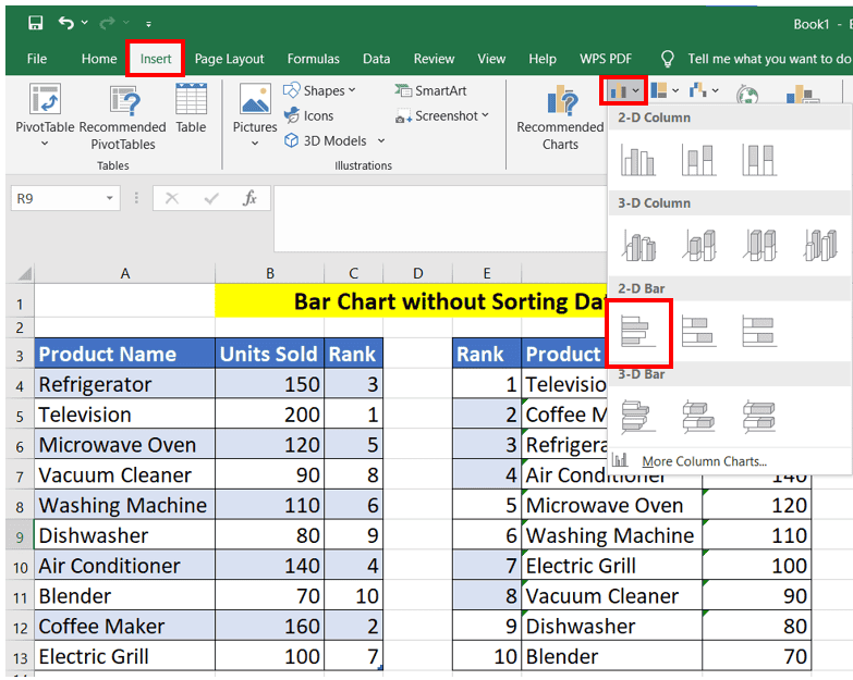
By following these steps, Excel will generate a 2-D bar chart that visually sorts the products according to the number of units sold in descending order while your original data set remains intact.
After creating the chart, it’s always a good practice to verify its dynamic nature. If we were to change a ‘Units Sold’ value, such as updating the units for ‘Electric Grill’ to a different number, the chart should automatically reflect this change and re-sort the bars accordingly.
Conclusion
In summary, by using Excel’s functions smartly, we’ve learned how to create a sorted bar chart without changing our original data. This is a neat trick to keep your data in place while still getting a clear picture of trends through visual analysis. It’s an easy and efficient way to make your data tell a story without disrupting the raw numbers.
Learn more about Excel and its functions through these helpful guides: